3 THE RELATIONAL MODEL

3THE RELATIONAL MODEL

TABLE: An arrangement of words, numbers, or signs, or combinations of them, as

in parallel columns, to exhibit a set of facts or relations in a definite, compact, and

comprehensive form; a synopsis or scheme.

—Webster’s Dictionary of the English Language

Codd proposed the relational data model in 1970. At that time most database systems

were based on one of two older data models (the hierarchical model and the network

model); the relational model revolutionized the database field and largely supplanted

these earlier models. Prototype relational database management systems were devel-

oped in pioneering research projects at IBM and UC-Berkeley by the mid-70s, and

several vendors were offering relational database products shortly thereafter. Today,

the relational model is by far the dominant data model and is the foundation for the

leading DBMS products, including IBM’s DB2 family, Informix, Oracle, Sybase, Mi-

crosoft’s Access and SQLServer, FoxBase, and Paradox. Relational database systems

are ubiquitous in the marketplace and represent a multibillion dollar industry.

The relational model is very simple and elegant; a database is a collection of one or more

relations, where each relation is a table with rows and columns. This simple tabular

representation enables even novice users to understand the contents of a database,

and it permits the use of simple, high-level languages to query the data. The major

advantages of the relational model over the older data models are its simple data

representation and the ease with which even complex queries can be expressed.

This chapter introduces the relational model and covers the following issues:

How is data represented?

What kinds of integrity constraints can be expressed?

How can data be created and modified?

How can data be manipulated and queried?

How do we obtain a database design in the relational model?

How are logical and physical data independence achieved?

51

52 Chapter 3

SQL: It was the query language of the pioneering System-R relational DBMS

developed at IBM. Over the years, SQL has become the most widely used language

for creating, manipulating, and querying relational DBMSs. Since many vendors

offer SQL products, there is a need for a standard that defines ‘official SQL.’

The existence of a standard allows users to measure a given vendor’s version of

SQL for completeness. It also allows users to distinguish SQL features that are

specific to one product from those that are standard; an application that relies on

non-standard features is less portable.

The first SQL standard was developed in 1986 by the American National Stan-

dards Institute (ANSI), and was called SQL-86. There was a minor revision in

1989 called SQL-89, and a major revision in 1992 called SQL-92. The Interna-

tional Standards Organization (ISO) collaborated with ANSI to develop SQL-92.

Most commercial DBMSs currently support SQL-92. An exciting development is

the imminent approval of SQL:1999, a major extension of SQL-92. While the cov-

erage of SQL in this book is based upon SQL-92, we will cover the main extensions

of SQL:1999 as well.

While we concentrate on the underlying concepts, we also introduce the Data Def-

inition Language (DDL) features of SQL-92, the standard language for creating,

manipulating, and querying data in a relational DBMS. This allows us to ground the

discussion firmly in terms of real database systems.

We discuss the concept of a relation in Section 3.1 and show how to create relations

using the SQL language. An important component of a data model is the set of

constructs it provides for specifying conditions that must be satisfied by the data. Such

conditions, called integrity constraints (ICs), enable the DBMS to reject operations that

might corrupt the data. We present integrity constraints in the relational model in

Section 3.2, along with a discussion of SQL support for ICs. We discuss how a DBMS

enforces integrity constraints in Section 3.3. In Section 3.4 we turn to the mechanism

for accessing and retrieving data from the database, query languages, and introduce

the querying features of SQL, which we examine in greater detail in a later chapter.

We then discuss the step of converting an ER diagram into a relational database schema

in Section 3.5. Finally, we introduce views, or tables defined using queries, in Section

3.6. Views can be used to define the external schema for a database and thus provide

the support for logical data independence in the relational model.

3.1 INTRODUCTION TO THE RELATIONAL MODEL

The main construct for representing data in the relational model is a relation. A

relation consists of a relation schema and a relation instance. The relation instance

The Relational Model 53

is a table, and the relation schema describes the column heads for the table. We first

describe the relation schema and then the relation instance. The schema specifies the

relation’s name, the name of each field (or column, or attribute), and the domain

of each field. A domain is referred to in a relation schema by the domain name and

has a set of associated values.

We use the example of student information in a university database from Chapter 1

to illustrate the parts of a relation schema:

Students(sid: string, name: string, login: string, age: integer, gpa: real)

This says, for instance, that the field named sid has a domain named string. The set

of values associated with domain string is the set of all character strings.

We now turn to the instances of a relation. An instance of a relation is a set of

tuples, also called records, in which each tuple has the same number of fields as the

relation schema. A relation instance can be thought of as a table in which each tuple

is a row, and all rows have the same number of fields. (The term relation instance is

often abbreviated to just relation, when there is no confusion with other aspects of a

relation such as its schema.)

An instance of the Students relation appears in Figure 3.1. The instance S1 contains

53831

53832

53650

53688

53666

50000 3.3

3.4

3.2

3.8

1.8

2.0

19

18

18

19

11

12

madayan@music

guldu@music

smith@math

smith@ee

jones@cs

dave@cs

Madayan

Guldu

Smith

Smith

Jones

Dave

sid age gpaloginname

TUPLES

(RECORDS, ROWS)

FIELDS (ATTRIBUTES, COLUMNS)

Field names

Figure 3.1 An Instance S1 of the Students Relation

six tuples and has, as we expect from the schema, five fields. Note that no two rows

are identical. This is a requirement of the relational model—each relation is defined

to be a set of unique tuples or rows.1 The order in which the rows are listed is not

important. Figure 3.2 shows the same relation instance. If the fields are named, as in

1In practice, commercial systems allow tables to have duplicate rows, but we will assume that arelation is indeed a set of tuples unless otherwise noted.

54 Chapter 3

sid name login age gpa

53831 Madayan madayan@music 11 1.8

53832 Guldu guldu@music 12 2.0

53688 Smith smith@ee 18 3.2

53650 Smith smith@math 19 3.8

53666 Jones jones@cs 18 3.4

50000 Dave dave@cs 19 3.3

Figure 3.2 An Alternative Representation of Instance S1 of Students

our schema definitions and figures depicting relation instances, the order of fields does

not matter either. However, an alternative convention is to list fields in a specific order

and to refer to a field by its position. Thus sid is field 1 of Students, login is field 3,

and so on. If this convention is used, the order of fields is significant. Most database

systems use a combination of these conventions. For example, in SQL the named fields

convention is used in statements that retrieve tuples, and the ordered fields convention

is commonly used when inserting tuples.

A relation schema specifies the domain of each field or column in the relation instance.

These domain constraints in the schema specify an important condition that we

want each instance of the relation to satisfy: The values that appear in a column must

be drawn from the domain associated with that column. Thus, the domain of a field

is essentially the type of that field, in programming language terms, and restricts the

values that can appear in the field.

More formally, let R(f1:D1, . . ., fn:Dn) be a relation schema, and for each fi, 1 ≤ i ≤ n,

let Domi be the set of values associated with the domain named Di. An instance of R

that satisfies the domain constraints in the schema is a set of tuples with n fields:

{ 〈f1 : d1, . . . , fn : dn〉 | d1 ∈ Dom1, . . . , dn ∈ Domn }

The angular brackets 〈. . .〉 identify the fields of a tuple. Using this notation, the first

Students tuple shown in Figure 3.1 is written as 〈sid: 50000, name: Dave, login:

dave@cs, age: 19, gpa: 3.3〉. The curly brackets {. . .} denote a set (of tuples, in this

definition). The vertical bar | should be read ‘such that,’ the symbol ∈ should be read

‘in,’ and the expression to the right of the vertical bar is a condition that must be

satisfied by the field values of each tuple in the set. Thus, an instance of R is defined

as a set of tuples. The fields of each tuple must correspond to the fields in the relation

schema.

Domain constraints are so fundamental in the relational model that we will henceforth

consider only relation instances that satisfy them; therefore, relation instance means

relation instance that satisfies the domain constraints in the relation schema.


The degree, also called arity, of a relation is the number of fields. The cardinality

of a relation instance is the number of tuples in it. In Figure 3.1, the degree of the

relation (the number of columns) is five, and the cardinality of this instance is six.

A relational database is a collection of relations with distinct relation names. The

relational database schema is the collection of schemas for the relations in the

database. For example, in Chapter 1, we discussed a university database with rela-

tions called Students, Faculty, Courses, Rooms, Enrolled, Teaches, and Meets In. An

instance of a relational database is a collection of relation instances, one per rela-

tion schema in the database schema; of course, each relation instance must satisfy the

domain constraints in its schema.

3.1.1 Creating and Modifying Relations Using SQL-92

The SQL-92 language standard uses the word table to denote relation, and we will

often follow this convention when discussing SQL. The subset of SQL that supports

the creation, deletion, and modification of tables is called the Data Definition Lan-

guage (DDL). Further, while there is a command that lets users define new domains,

analogous to type definition commands in a programming language, we postpone a dis-

cussion of domain definition until Section 5.11. For now, we will just consider domains

that are built-in types, such as integer.

The CREATE TABLE statement is used to define a new table.2 To create the Students

relation, we can use the following statement:

CREATE TABLE Students ( sid CHAR(20),

name CHAR(30),

login CHAR(20),

age INTEGER,

gpa REAL )

Tuples are inserted using the INSERT command. We can insert a single tuple into the

Students table as follows:

INSERT

INTO Students (sid, name, login, age, gpa)

VALUES (53688, ‘Smith’, ‘smith@ee’, 18, 3.2)

We can optionally omit the list of column names in the INTO clause and list the values

in the appropriate order, but it is good style to be explicit about column names.

2SQL also provides statements to destroy tables and to change the columns associated with a table;we discuss these in Section 3.7.

56 Chapter 3

We can delete tuples using the DELETE command. We can delete all Students tuples

with name equal to Smith using the command:

DELETE

FROM Students S

WHERE S.name = ‘Smith’

We can modify the column values in an existing row using the UPDATE command. For

example, we can increment the age and decrement the gpa of the student with sid

53688:

UPDATE Students S

SET S.age = S.age + 1, S.gpa = S.gpa - 1

WHERE S.sid = 53688

These examples illustrate some important points. The WHERE clause is applied first

and determines which rows are to be modified. The SET clause then determines how

these rows are to be modified. If the column that is being modified is also used to

determine the new value, the value used in the expression on the right side of equals

(=) is the old value, that is, before the modification. To illustrate these points further,

consider the following variation of the previous query:

UPDATE Students S

SET S.gpa = S.gpa - 0.1

WHERE S.gpa >= 3.3

If this query is applied on the instance S1 of Students shown in Figure 3.1, we obtain

the instance shown in Figure 3.3.








Figure 3.3 Students Instance S1 after Update

3.2 INTEGRITY CONSTRAINTS OVER RELATIONS

A database is only as good as the information stored in it, and a DBMS must therefore

help prevent the entry of incorrect information. An integrity constraint (IC) is a


condition that is specified on a database schema, and restricts the data that can be

stored in an instance of the database. If a database instance satisfies all the integrity

constraints specified on the database schema, it is a legal instance. A DBMS enforces

integrity constraints, in that it permits only legal instances to be stored in the database.

Integrity constraints are specified and enforced at different times:

1. When the DBA or end user defines a database schema, he or she specifies the ICs

that must hold on any instance of this database.

2. When a database application is run, the DBMS checks for violations and disallows

changes to the data that violate the specified ICs. (In some situations, rather than

disallow the change, the DBMS might instead make some compensating changes

to the data to ensure that the database instance satisfies all ICs. In any case,

changes to the database are not allowed to create an instance that violates any

IC.)

Many kinds of integrity constraints can be specified in the relational model. We have

already seen one example of an integrity constraint in the domain constraints associated

with a relation schema (Section 3.1). In general, other kinds of constraints can be

specified as well; for example, no two students have the same sid value. In this section

we discuss the integrity constraints, other than domain constraints, that a DBA or

user can specify in the relational model.

3.2.1 Key Constraints

Consider the Students relation and the constraint that no two students have the same

student id. This IC is an example of a key constraint. A key constraint is a statement

that a certain minimal subset of the fields of a relation is a unique identifier for a tuple.

A set of fields that uniquely identifies a tuple according to a key constraint is called

a candidate key for the relation; we often abbreviate this to just key. In the case of

the Students relation, the (set of fields containing just the) sid field is a candidate key.

Let us take a closer look at the above definition of a (candidate) key. There are two

parts to the definition:3

1. Two distinct tuples in a legal instance (an instance that satisfies all ICs, including

the key constraint) cannot have identical values in all the fields of a key.

2. No subset of the set of fields in a key is a unique identifier for a tuple.

3The term key is rather overworked. In the context of access methods, we speak of search keys,which are quite different.

58 Chapter 3

The first part of the definition means that in any legal instance, the values in the key

fields uniquely identify a tuple in the instance. When specifying a key constraint, the

DBA or user must be sure that this constraint will not prevent them from storing a

‘correct’ set of tuples. (A similar comment applies to the specification of other kinds

of ICs as well.) The notion of ‘correctness’ here depends upon the nature of the data

being stored. For example, several students may have the same name, although each

student has a unique student id. If the name field is declared to be a key, the DBMS

will not allow the Students relation to contain two tuples describing different students

with the same name!

The second part of the definition means, for example, that the set of fields {sid, name}

is not a key for Students, because this set properly contains the key {sid}. The set

{sid, name} is an example of a superkey, which is a set of fields that contains a key.

Look again at the instance of the Students relation in Figure 3.1. Observe that two

different rows always have different sid values; sid is a key and uniquely identifies a

tuple. However, this does not hold for nonkey fields. For example, the relation contains

two rows with Smith in the name field.

Note that every relation is guaranteed to have a key. Since a relation is a set of tuples,

the set of all fields is always a superkey. If other constraints hold, some subset of the

fields may form a key, but if not, the set of all fields is a key.

A relation may have several candidate keys. For example, the login and age fields of

the Students relation may, taken together, also identify students uniquely. That is,

{login, age} is also a key. It may seem that login is a key, since no two rows in the

example instance have the same login value. However, the key must identify tuples

uniquely in all possible legal instances of the relation. By stating that {login, age} is

a key, the user is declaring that two students may have the same login or age, but not

both.

Out of all the available candidate keys, a database designer can identify a primary

key. Intuitively, a tuple can be referred to from elsewhere in the database by storing

the values of its primary key fields. For example, we can refer to a Students tuple by

storing its sid value. As a consequence of referring to student tuples in this manner,

tuples are frequently accessed by specifying their sid value. In principle, we can use

any key, not just the primary key, to refer to a tuple. However, using the primary key is

preferable because it is what the DBMS expects—this is the significance of designating

a particular candidate key as a primary key—and optimizes for. For example, the

DBMS may create an index with the primary key fields as the search key, to make

the retrieval of a tuple given its primary key value efficient. The idea of referring to a

tuple is developed further in the next section.


Specifying Key Constraints in SQL-92

In SQL we can declare that a subset of the columns of a table constitute a key by

using the UNIQUE constraint. At most one of these ‘candidate’ keys can be declared

to be a primary key, using the PRIMARY KEY constraint. (SQL does not require that

such constraints be declared for a table.)

Let us revisit our example table definition and specify key information:

CREATE TABLE Students ( sid CHAR(20),

name CHAR(30),

login CHAR(20),

age INTEGER,

gpa REAL,

UNIQUE (name, age),

CONSTRAINT StudentsKey PRIMARY KEY (sid) )

This definition says that sid is the primary key and that the combination of name and

age is also a key. The definition of the primary key also illustrates how we can name

a constraint by preceding it with CONSTRAINT constraint-name. If the constraint is

violated, the constraint name is returned and can be used to identify the error.

3.2.2 Foreign Key Constraints

Sometimes the information stored in a relation is linked to the information stored in

another relation. If one of the relations is modified, the other must be checked, and

perhaps modified, to keep the data consistent. An IC involving both relations must

be specified if a DBMS is to make such checks. The most common IC involving two

relations is a foreign key constraint.

Suppose that in addition to Students, we have a second relation:

Enrolled(sid: string, cid: string, grade: string)

To ensure that only bona fide students can enroll in courses, any value that appears in

the sid field of an instance of the Enrolled relation should also appear in the sid field

of some tuple in the Students relation. The sid field of Enrolled is called a foreign

key and refers to Students. The foreign key in the referencing relation (Enrolled, in

our example) must match the primary key of the referenced relation (Students), i.e.,

it must have the same number of columns and compatible data types, although the

column names can be different.

This constraint is illustrated in Figure 3.4. As the figure shows, there may well be

some students who are not referenced from Enrolled (e.g., the student with sid=50000).

60 Chapter 3

However, every sid value that appears in the instance of the Enrolled table appears in

the primary key column of a row in the Students table.

cid grade sid

53831

53832

53650

53688

53666

50000Carnatic101

Reggae203

Topology112

History105

53831

53832

53650

53666

3.3

3.4

3.2

3.8

1.8

2.0

19

18

18

19

11

12

madayan@music

guldu@music

smith@math

smith@ee

jones@cs

dave@cs

Madayan

Guldu

Smith

Smith

Jones

DaveC

B

A

B

Enrolled (Referencing relation) (Referenced relation)Students

Primary keyForeign key

sid age gpaloginname

Figure 3.4 Referential Integrity

If we try to insert the tuple 〈55555, Art104, A〉 into E1, the IC is violated because

there is no tuple in S1 with the id 55555; the database system should reject such

an insertion. Similarly, if we delete the tuple 〈53666, Jones, jones@cs, 18, 3.4〉 from

S1, we violate the foreign key constraint because the tuple 〈53666, History105, B〉

in E1 contains sid value 53666, the sid of the deleted Students tuple. The DBMS

should disallow the deletion or, perhaps, also delete the Enrolled tuple that refers to

the deleted Students tuple. We discuss foreign key constraints and their impact on

updates in Section 3.3.

Finally, we note that a foreign key could refer to the same relation. For example,

we could extend the Students relation with a column called partner and declare this

column to be a foreign key referring to Students. Intuitively, every student could then

have a partner, and the partner field contains the partner’s sid. The observant reader

will no doubt ask, “What if a student does not (yet) have a partner?” This situation

is handled in SQL by using a special value called null. The use of null in a field of a

tuple means that value in that field is either unknown or not applicable (e.g., we do not

know the partner yet, or there is no partner). The appearance of null in a foreign key

field does not violate the foreign key constraint. However, null values are not allowed

to appear in a primary key field (because the primary key fields are used to identify a

tuple uniquely). We will discuss null values further in Chapter 5.

Specifying Foreign Key Constraints in SQL-92

Let us define Enrolled(sid: string, cid: string, grade: string):

CREATE TABLE Enrolled ( sid CHAR(20),


cid CHAR(20),

grade CHAR(10),

PRIMARY KEY (sid, cid),

FOREIGN KEY (sid) REFERENCES Students )

The foreign key constraint states that every sid value in Enrolled must also appear in

Students, that is, sid in Enrolled is a foreign key referencing Students. Incidentally,

the primary key constraint states that a student has exactly one grade for each course

that he or she is enrolled in. If we want to record more than one grade per student

per course, we should change the primary key constraint.

3.2.3 General Constraints

Domain, primary key, and foreign key constraints are considered to be a fundamental

part of the relational data model and are given special attention in most commercial

systems. Sometimes, however, it is necessary to specify more general constraints.

For example, we may require that student ages be within a certain range of values;

given such an IC specification, the DBMS will reject inserts and updates that violate

the constraint. This is very useful in preventing data entry errors. If we specify that

all students must be at least 16 years old, the instance of Students shown in Figure

3.1 is illegal because two students are underage. If we disallow the insertion of these

two tuples, we have a legal instance, as shown in Figure 3.5.





Figure 3.5 An Instance S2 of the Students Relation

The IC that students must be older than 16 can be thought of as an extended domain

constraint, since we are essentially defining the set of permissible age values more strin-

gently than is possible by simply using a standard domain such as integer. In general,

however, constraints that go well beyond domain, key, or foreign key constraints can

be specified. For example, we could require that every student whose age is greater

than 18 must have a gpa greater than 3.

Current relational database systems support such general constraints in the form of

table constraints and assertions. Table constraints are associated with a single table

and are checked whenever that table is modified. In contrast, assertions involve several

62 Chapter 3

tables and are checked whenever any of these tables is modified. Both table constraints

and assertions can use the full power of SQL queries to specify the desired restriction.

We discuss SQL support for table constraints and assertions in Section 5.11 because a

full appreciation of their power requires a good grasp of SQL’s query capabilities.

3.3 ENFORCING INTEGRITY CONSTRAINTS

As we observed earlier, ICs are specified when a relation is created and enforced when

a relation is modified. The impact of domain, PRIMARY KEY, and UNIQUE constraints

is straightforward: if an insert, delete, or update command causes a violation, it is

rejected. Potential IC violation is generally checked at the end of each SQL statement

execution, although it can be deferred until the end of the transaction executing the

statement, as we will see in Chapter 18.

Consider the instance S1 of Students shown in Figure 3.1. The following insertion

violates the primary key constraint because there is already a tuple with the sid 53688,

and it will be rejected by the DBMS:

INSERT


VALUES (53688, ‘Mike’, ‘mike@ee’, 17, 3.4)

The following insertion violates the constraint that the primary key cannot contain

null:

INSERT


VALUES (null, ‘Mike’, ‘mike@ee’, 17, 3.4)

Of course, a similar problem arises whenever we try to insert a tuple with a value in

a field that is not in the domain associated with that field, i.e., whenever we violate

a domain constraint. Deletion does not cause a violation of domain, primary key or

unique constraints. However, an update can cause violations, similar to an insertion:

UPDATE Students S

SET S.sid = 50000

WHERE S.sid = 53688

This update violates the primary key constraint because there is already a tuple with

sid 50000.

The impact of foreign key constraints is more complex because SQL sometimes tries to

rectify a foreign key constraint violation instead of simply rejecting the change. We will


discuss the referential integrity enforcement steps taken by the DBMS in terms

of our Enrolled and Students tables, with the foreign key constraint that Enrolled.sid

is a reference to (the primary key of) Students.

In addition to the instance S1 of Students, consider the instance of Enrolled shown

in Figure 3.4. Deletions of Enrolled tuples do not violate referential integrity, but

insertions of Enrolled tuples could. The following insertion is illegal because there is

no student with sid 51111:

INSERT

INTO Enrolled (cid, grade, sid)

VALUES (‘Hindi101’, ‘B’, 51111)

On the other hand, insertions of Students tuples do not violate referential integrity

although deletions could. Further, updates on either Enrolled or Students that change

the sid value could potentially violate referential integrity.

SQL-92 provides several alternative ways to handle foreign key violations. We must

consider three basic questions:

1. What should we do if an Enrolled row is inserted, with a sid column value that

does not appear in any row of the Students table?

In this case the INSERT command is simply rejected.

2. What should we do if a Students row is deleted?

The options are:

Delete all Enrolled rows that refer to the deleted Students row.

Disallow the deletion of the Students row if an Enrolled row refers to it.

Set the sid column to the sid of some (existing) ‘default’ student, for every

Enrolled row that refers to the deleted Students row.

For every Enrolled row that refers to it, set the sid column to null. In our

example, this option conflicts with the fact that sid is part of the primary

key of Enrolled and therefore cannot be set to null. Thus, we are limited to

the first three options in our example, although this fourth option (setting

the foreign key to null) is available in the general case.

3. What should we do if the primary key value of a Students row is updated?

The options here are similar to the previous case.

SQL-92 allows us to choose any of the four options on DELETE and UPDATE. For exam-

ple, we can specify that when a Students row is deleted, all Enrolled rows that refer to

it are to be deleted as well, but that when the sid column of a Students row is modified,

this update is to be rejected if an Enrolled row refers to the modified Students row:

64 Chapter 3

CREATE TABLE Enrolled ( sid CHAR(20),

cid CHAR(20),

grade CHAR(10),

PRIMARY KEY (sid, cid),

FOREIGN KEY (sid) REFERENCES Students

ON DELETE CASCADE

ON UPDATE NO ACTION )

The options are specified as part of the foreign key declaration. The default option is

NO ACTION, which means that the action (DELETE or UPDATE) is to be rejected. Thus,

the ON UPDATE clause in our example could be omitted, with the same effect. The

CASCADE keyword says that if a Students row is deleted, all Enrolled rows that refer

to it are to be deleted as well. If the UPDATE clause specified CASCADE, and the sid

column of a Students row is updated, this update is also carried out in each Enrolled

row that refers to the updated Students row.

If a Students row is deleted, we can switch the enrollment to a ‘default’ student by using

ON DELETE SET DEFAULT. The default student is specified as part of the definition of

the sid field in Enrolled; for example, sid CHAR(20) DEFAULT ‘53666’. Although the

specification of a default value is appropriate in some situations (e.g., a default parts

supplier if a particular supplier goes out of business), it is really not appropriate to

switch enrollments to a default student. The correct solution in this example is to also

delete all enrollment tuples for the deleted student (that is, CASCADE), or to reject the

update.

SQL also allows the use of null as the default value by specifying ON DELETE SET NULL.

3.4 QUERYING RELATIONAL DATA

A relational database query (query, for short) is a question about the data, and the

answer consists of a new relation containing the result. For example, we might want

to find all students younger than 18 or all students enrolled in Reggae203. A query

language is a specialized language for writing queries.

SQL is the most popular commercial query language for a relational DBMS. We now

present some SQL examples that illustrate how easily relations can be queried. Con-

sider the instance of the Students relation shown in Figure 3.1. We can retrieve rows

corresponding to students who are younger than 18 with the following SQL query:

SELECT *

FROM Students S

WHERE S.age < 18


The symbol * means that we retain all fields of selected tuples in the result. To

understand this query, think of S as a variable that takes on the value of each tuple

in Students, one tuple after the other. The condition S.age < 18 in the WHERE clause

specifies that we want to select only tuples in which the age field has a value less than

18. This query evaluates to the relation shown in Figure 3.6.




Figure 3.6 Students with age < 18 on Instance S1

This example illustrates that the domain of a field restricts the operations that are

permitted on field values, in addition to restricting the values that can appear in the

field. The condition S.age < 18 involves an arithmetic comparison of an age value with

an integer and is permissible because the domain of age is the set of integers. On the

other hand, a condition such as S.age = S.sid does not make sense because it compares

an integer value with a string value, and this comparison is defined to fail in SQL; a

query containing this condition will produce no answer tuples.

In addition to selecting a subset of tuples, a query can extract a subset of the fields

of each selected tuple. We can compute the names and logins of students who are

younger than 18 with the following query:

SELECT S.name, S.login

FROM Students S

WHERE S.age < 18

Figure 3.7 shows the answer to this query; it is obtained by applying the selection

to the instance S1 of Students (to get the relation shown in Figure 3.6), followed by

removing unwanted fields. Note that the order in which we perform these operations

does matter—if we remove unwanted fields first, we cannot check the condition S.age

< 18, which involves one of those fields.

We can also combine information in the Students and Enrolled relations. If we want to

obtain the names of all students who obtained an A and the id of the course in which

they got an A, we could write the following query:

SELECT S.name, E.cid

FROM Students S, Enrolled E

WHERE S.sid = E.sid AND E.grade = ‘A’

66 Chapter 3

DISTINCT types in SQL: A comparison of two values drawn from different do-

mains should fail, even if the values are ‘compatible’ in the sense that both are

numeric or both are string values etc. For example, if salary and age are two dif-

ferent domains whose values are represented as integers, a comparison of a salary

value with an age value should fail. Unfortunately, SQL-92’s support for the con-

cept of domains does not go this far: We are forced to define salary and age as

integer types and the comparison S < A will succeed when S is bound to the

salary value 25 and A is bound to the age value 50. The latest version of the SQL

standard, called SQL:1999, addresses this problem, and allows us to define salary

and age as DISTINCT types even though their values are represented as integers.

Many systems, e.g., Informix UDS and IBM DB2, already support this feature.

name login

Madayan madayan@music

Guldu guldu@music

Figure 3.7 Names and Logins of Students under 18

This query can be understood as follows: “If there is a Students tuple S and an Enrolled

tuple E such that S.sid = E.sid (so that S describes the student who is enrolled in E)

and E.grade = ‘A’, then print the student’s name and the course id.” When evaluated

on the instances of Students and Enrolled in Figure 3.4, this query returns a single

tuple, 〈Smith, Topology112〉.

We will cover relational queries, and SQL in particular, in more detail in subsequent

chapters.

3.5 LOGICAL DATABASE DESIGN: ER TO RELATIONAL

The ER model is convenient for representing an initial, high-level database design.

Given an ER diagram describing a database, there is a standard approach to generating

a relational database schema that closely approximates the ER design. (The translation

is approximate to the extent that we cannot capture all the constraints implicit in the

ER design using SQL-92, unless we use certain SQL-92 constraints that are costly to

check.) We now describe how to translate an ER diagram into a collection of tables

with associated constraints, i.e., a relational database schema.


3.5.1 Entity Sets to Tables

An entity set is mapped to a relation in a straightforward way: Each attribute of the

entity set becomes an attribute of the table. Note that we know both the domain of

each attribute and the (primary) key of an entity set.

Consider the Employees entity set with attributes ssn, name, and lot shown in Figure

3.8. A possible instance of the Employees entity set, containing three Employees

Employees

ssn

name

lot

Figure 3.8 The Employees Entity Set

entities, is shown in Figure 3.9 in a tabular format.

ssn name lot

123-22-3666 Attishoo 48

231-31-5368 Smiley 22

131-24-3650 Smethurst 35

Figure 3.9 An Instance of the Employees Entity Set

The following SQL statement captures the preceding information, including the domain

constraints and key information:

CREATE TABLE Employees ( ssn CHAR(11),

name CHAR(30),

lot INTEGER,

PRIMARY KEY (ssn) )

3.5.2 Relationship Sets (without Constraints) to Tables

A relationship set, like an entity set, is mapped to a relation in the relational model.

We begin by considering relationship sets without key and participation constraints,

and we discuss how to handle such constraints in subsequent sections. To represent

a relationship, we must be able to identify each participating entity and give values

68 Chapter 3

to the descriptive attributes of the relationship. Thus, the attributes of the relation

include:

The primary key attributes of each participating entity set, as foreign key fields.

The descriptive attributes of the relationship set.

The set of nondescriptive attributes is a superkey for the relation. If there are no key

constraints (see Section 2.4.1), this set of attributes is a candidate key.

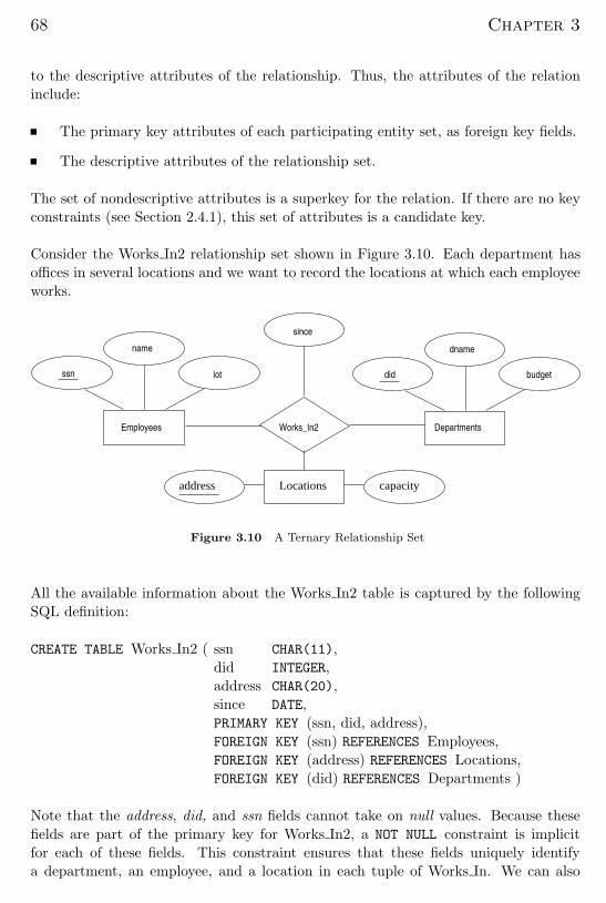
Consider the Works In2 relationship set shown in Figure 3.10. Each department has

offices in several locations and we want to record the locations at which each employee

works.

dname

budgetdid

since

name

Employees

ssn lot

Locations

Departments

capacityaddress

Works_In2

Figure 3.10 A Ternary Relationship Set

All the available information about the Works In2 table is captured by the following

SQL definition:

CREATE TABLE Works In2 ( ssn CHAR(11),

did INTEGER,

address CHAR(20),

since DATE,

PRIMARY KEY (ssn, did, address),

FOREIGN KEY (ssn) REFERENCES Employees,

FOREIGN KEY (address) REFERENCES Locations,

FOREIGN KEY (did) REFERENCES Departments )

Note that the address, did, and ssn fields cannot take on null values. Because these

fields are part of the primary key for Works In2, a NOT NULL constraint is implicit

for each of these fields. This constraint ensures that these fields uniquely identify

a department, an employee, and a location in each tuple of Works In. We can also


specify that a particular action is desired when a referenced Employees, Departments

or Locations tuple is deleted, as explained in the discussion of integrity constraints in

Section 3.2. In this chapter we assume that the default action is appropriate except

for situations in which the semantics of the ER diagram require some other action.

Finally, consider the Reports To relationship set shown in Figure 3.11. The role in-

Reports_To

name

Employees

subordinatesupervisor

ssn lot

Figure 3.11 The Reports To Relationship Set

dicators supervisor and subordinate are used to create meaningful field names in the

CREATE statement for the Reports To table:

CREATE TABLE Reports To (

supervisor ssn CHAR(11),

subordinate ssn CHAR(11),

PRIMARY KEY (supervisor ssn, subordinate ssn),

FOREIGN KEY (supervisor ssn) REFERENCES Employees(ssn),

FOREIGN KEY (subordinate ssn) REFERENCES Employees(ssn) )

Observe that we need to explicitly name the referenced field of Employees because the

field name differs from the name(s) of the referring field(s).

3.5.3 Translating Relationship Sets with Key Constraints

If a relationship set involves n entity sets and some m of them are linked via arrows

in the ER diagram, the key for any one of these m entity sets constitutes a key for

the relation to which the relationship set is mapped. Thus we have m candidate keys,

and one of these should be designated as the primary key. The translation discussed

in Section 2.3 from relationship sets to a relation can be used in the presence of key

constraints, taking into account this point about keys.

70 Chapter 3

Consider the relationship set Manages shown in Figure 3.12. The table corresponding

name dname

budgetdid

since

ManagesEmployees Departments

ssn lot

Figure 3.12 Key Constraint on Manages

to Manages has the attributes ssn, did, since. However, because each department has

at most one manager, no two tuples can have the same did value but differ on the ssn

value. A consequence of this observation is that did is itself a key for Manages; indeed,

the set did, ssn is not a key (because it is not minimal). The Manages relation can be

defined using the following SQL statement:

CREATE TABLE Manages ( ssn CHAR(11),

did INTEGER,

since DATE,

PRIMARY KEY (did),

FOREIGN KEY (ssn) REFERENCES Employees,

FOREIGN KEY (did) REFERENCES Departments )

A second approach to translating a relationship set with key constraints is often su-

perior because it avoids creating a distinct table for the relationship set. The idea

is to include the information about the relationship set in the table corresponding to

the entity set with the key, taking advantage of the key constraint. In the Manages

example, because a department has at most one manager, we can add the key fields of

the Employees tuple denoting the manager and the since attribute to the Departments

tuple.

This approach eliminates the need for a separate Manages relation, and queries asking

for a department’s manager can be answered without combining information from two

relations. The only drawback to this approach is that space could be wasted if several

departments have no managers. In this case the added fields would have to be filled

with null values. The first translation (using a separate table for Manages) avoids this

inefficiency, but some important queries require us to combine information from two

relations, which can be a slow operation.

The following SQL statement, defining a Dept Mgr relation that captures the informa-

tion in both Departments and Manages, illustrates the second approach to translating

relationship sets with key constraints:


CREATE TABLE Dept Mgr ( did INTEGER,

dname CHAR(20),

budget REAL,

ssn CHAR(11),

since DATE,

PRIMARY KEY (did),

FOREIGN KEY (ssn) REFERENCES Employees )

Note that ssn can take on null values.

This idea can be extended to deal with relationship sets involving more than two entity

sets. In general, if a relationship set involves n entity sets and some m of them are

linked via arrows in the ER diagram, the relation corresponding to any one of the m

sets can be augmented to capture the relationship.

We discuss the relative merits of the two translation approaches further after consid-

ering how to translate relationship sets with participation constraints into tables.

3.5.4 Translating Relationship Sets with Participation Constraints

Consider the ER diagram in Figure 3.13, which shows two relationship sets, Manages

and Works In.

name dname

budgetdid

since

Manages

name dname

budgetdid

since

Manages

since

DepartmentsEmployees

ssn

Works_In

lot

Figure 3.13 Manages and Works In

72 Chapter 3

Every department is required to have a manager, due to the participation constraint,

and at most one manager, due to the key constraint. The following SQL statement

reflects the second translation approach discussed in Section 3.5.3, and uses the key

constraint:

CREATE TABLE Dept Mgr ( did INTEGER,

dname CHAR(20),

budget REAL,

ssn CHAR(11) NOT NULL,

since DATE,

PRIMARY KEY (did),

FOREIGN KEY (ssn) REFERENCES Employees

ON DELETE NO ACTION )

It also captures the participation constraint that every department must have a man-

ager: Because ssn cannot take on null values, each tuple of Dept Mgr identifies a tuple

in Employees (who is the manager). The NO ACTION specification, which is the default

and need not be explicitly specified, ensures that an Employees tuple cannot be deleted

while it is pointed to by a Dept Mgr tuple. If we wish to delete such an Employees

tuple, we must first change the Dept Mgr tuple to have a new employee as manager.

(We could have specified CASCADE instead of NO ACTION, but deleting all information

about a department just because its manager has been fired seems a bit extreme!)

The constraint that every department must have a manager cannot be captured using

the first translation approach discussed in Section 3.5.3. (Look at the definition of

Manages and think about what effect it would have if we added NOT NULL constraints

to the ssn and did fields. Hint: The constraint would prevent the firing of a manager,

but does not ensure that a manager is initially appointed for each department!) This

situation is a strong argument in favor of using the second approach for one-to-many

relationships such as Manages, especially when the entity set with the key constraint

also has a total participation constraint.

Unfortunately, there are many participation constraints that we cannot capture using

SQL-92, short of using table constraints or assertions. Table constraints and assertions

can be specified using the full power of the SQL query language (as discussed in

Section 5.11) and are very expressive, but also very expensive to check and enforce.

For example, we cannot enforce the participation constraints on the Works In relation

without using these general constraints. To see why, consider the Works In relation

obtained by translating the ER diagram into relations. It contains fields ssn and

did, which are foreign keys referring to Employees and Departments. To ensure total

participation of Departments in Works In, we have to guarantee that every did value in

Departments appears in a tuple of Works In. We could try to guarantee this condition

by declaring that did in Departments is a foreign key referring to Works In, but this

is not a valid foreign key constraint because did is not a candidate key for Works In.


To ensure total participation of Departments in Works In using SQL-92, we need an

assertion. We have to guarantee that every did value in Departments appears in a

tuple of Works In; further, this tuple of Works In must also have non null values in

the fields that are foreign keys referencing other entity sets involved in the relationship

(in this example, the ssn field). We can ensure the second part of this constraint by

imposing the stronger requirement that ssn in Works In cannot contain null values.

(Ensuring that the participation of Employees in Works In is total is symmetric.)

Another constraint that requires assertions to express in SQL is the requirement that

each Employees entity (in the context of the Manages relationship set) must manage

at least one department.

In fact, the Manages relationship set exemplifies most of the participation constraints

that we can capture using key and foreign key constraints. Manages is a binary rela-

tionship set in which exactly one of the entity sets (Departments) has a key constraint,

and the total participation constraint is expressed on that entity set.

We can also capture participation constraints using key and foreign key constraints in

one other special situation: a relationship set in which all participating entity sets have

key constraints and total participation. The best translation approach in this case is

to map all the entities as well as the relationship into a single table; the details are

straightforward.

3.5.5 Translating Weak Entity Sets

A weak entity set always participates in a one-to-many binary relationship and has a

key constraint and total participation. The second translation approach discussed in

Section 3.5.3 is ideal in this case, but we must take into account the fact that the weak

entity has only a partial key. Also, when an owner entity is deleted, we want all owned

weak entities to be deleted.

Consider the Dependents weak entity set shown in Figure 3.14, with partial key pname.

A Dependents entity can be identified uniquely only if we take the key of the owning

Employees entity and the pname of the Dependents entity, and the Dependents entity

must be deleted if the owning Employees entity is deleted.

We can capture the desired semantics with the following definition of the Dep Policy

relation:

CREATE TABLE Dep Policy ( pname CHAR(20),

age INTEGER,

cost REAL,

ssn CHAR(11),

74 Chapter 3

name

agepname

DependentsEmployees

ssn

Policy

costlot

Figure 3.14 The Dependents Weak Entity Set

PRIMARY KEY (pname, ssn),


ON DELETE CASCADE )

Observe that the primary key is 〈pname, ssn〉, since Dependents is a weak entity. This

constraint is a change with respect to the translation discussed in Section 3.5.3. We

have to ensure that every Dependents entity is associated with an Employees entity

(the owner), as per the total participation constraint on Dependents. That is, ssn

cannot be null. This is ensured because ssn is part of the primary key. The CASCADE

option ensures that information about an employee’s policy and dependents is deleted

if the corresponding Employees tuple is deleted.

3.5.6 Translating Class Hierarchies

We present the two basic approaches to handling ISA hierarchies by applying them to

the ER diagram shown in Figure 3.15:

name

ISA

ssn

EmployeeEmployees

Hourly_Emps Contract_Emps

lot

contractidhours_worked

hourly_wages

Figure 3.15 Class Hierarchy


1. We can map each of the entity sets Employees, Hourly Emps, and Contract Emps

to a distinct relation. The Employees relation is created as in Section 2.2. We

discuss Hourly Emps here; Contract Emps is handled similarly. The relation for

Hourly Emps includes the hourly wages and hours worked attributes of Hourly Emps.

It also contains the key attributes of the superclass (ssn, in this example), which

serve as the primary key for Hourly Emps, as well as a foreign key referencing

the superclass (Employees). For each Hourly Emps entity, the value of the name

and lot attributes are stored in the corresponding row of the superclass (Employ-

ees). Note that if the superclass tuple is deleted, the delete must be cascaded to

Hourly Emps.

2. Alternatively, we can create just two relations, corresponding to Hourly Emps

and Contract Emps. The relation for Hourly Emps includes all the attributes

of Hourly Emps as well as all the attributes of Employees (i.e., ssn, name, lot,

hourly wages, hours worked).

The first approach is general and is always applicable. Queries in which we want to

examine all employees and do not care about the attributes specific to the subclasses

are handled easily using the Employees relation. However, queries in which we want

to examine, say, hourly employees, may require us to combine Hourly Emps (or Con-

tract Emps, as the case may be) with Employees to retrieve name and lot.

The second approach is not applicable if we have employees who are neither hourly

employees nor contract employees, since there is no way to store such employees. Also,

if an employee is both an Hourly Emps and a Contract Emps entity, then the name

and lot values are stored twice. This duplication can lead to some of the anomalies

that we discuss in Chapter 15. A query that needs to examine all employees must now

examine two relations. On the other hand, a query that needs to examine only hourly

employees can now do so by examining just one relation. The choice between these

approaches clearly depends on the semantics of the data and the frequency of common

operations.

In general, overlap and covering constraints can be expressed in SQL-92 only by using

assertions.

3.5.7 Translating ER Diagrams with Aggregation

Translating aggregation into the relational model is easy because there is no real dis-

tinction between entities and relationships in the relational model.

Consider the ER diagram shown in Figure 3.16. The Employees, Projects, and De-

partments entity sets and the Sponsors relationship set are mapped as described in

previous sections. For the Monitors relationship set, we create a relation with the

following attributes: the key attributes of Employees (ssn), the key attributes of Spon-

76 Chapter 3

until

since

name

budgetdidpid

started_on

pbudget

dname

ssn

DepartmentsProjects Sponsors

Employees

Monitors

lot

Figure 3.16 Aggregation

sors (did, pid), and the descriptive attributes of Monitors (until). This translation is

essentially the standard mapping for a relationship set, as described in Section 3.5.2.

There is a special case in which this translation can be refined further by dropping

the Sponsors relation. Consider the Sponsors relation. It has attributes pid, did, and

since, and in general we need it (in addition to Monitors) for two reasons:

1. We have to record the descriptive attributes (in our example, since) of the Sponsors

relationship.

2. Not every sponsorship has a monitor, and thus some 〈pid, did〉 pairs in the Spon-

sors relation may not appear in the Monitors relation.

However, if Sponsors has no descriptive attributes and has total participation in Mon-

itors, every possible instance of the Sponsors relation can be obtained by looking at

the 〈pid, did〉 columns of the Monitors relation. Thus, we need not store the Sponsors

relation in this case.

3.5.8 ER to Relational: Additional Examples *

Consider the ER diagram shown in Figure 3.17. We can translate this ER diagram

into the relational model as follows, taking advantage of the key constraints to combine

Purchaser information with Policies and Beneficiary information with Dependents:


name

agepname

DependentsEmployees

ssn

policyid cost

Beneficiary

lot

Policies

Purchaser

Figure 3.17 Policy Revisited

CREATE TABLE Policies ( policyid INTEGER,

cost REAL,

ssn CHAR(11) NOT NULL,

PRIMARY KEY (policyid),


ON DELETE CASCADE )

CREATE TABLE Dependents ( pname CHAR(20),

age INTEGER,

policyid INTEGER,

PRIMARY KEY (pname, policyid),

FOREIGN KEY (policyid) REFERENCES Policies

ON DELETE CASCADE )

Notice how the deletion of an employee leads to the deletion of all policies owned by

the employee and all dependents who are beneficiaries of those policies. Further, each

dependent is required to have a covering policy—because policyid is part of the primary

key of Dependents, there is an implicit NOT NULL constraint. This model accurately

reflects the participation constraints in the ER diagram and the intended actions when

an employee entity is deleted.

In general, there could be a chain of identifying relationships for weak entity sets. For

example, we assumed that policyid uniquely identifies a policy. Suppose that policyid

only distinguishes the policies owned by a given employee; that is, policyid is only a

partial key and Policies should be modeled as a weak entity set. This new assumption

78 Chapter 3

about policyid does not cause much to change in the preceding discussion. In fact,

the only changes are that the primary key of Policies becomes 〈policyid, ssn〉, and as

a consequence, the definition of Dependents changes—a field called ssn is added and

becomes part of both the primary key of Dependents and the foreign key referencing

Policies:

CREATE TABLE Dependents ( pname CHAR(20),

ssn CHAR(11),

age INTEGER,

policyid INTEGER NOT NULL,

PRIMARY KEY (pname, policyid, ssn),

FOREIGN KEY (policyid, ssn) REFERENCES Policies

ON DELETE CASCADE)

3.6 INTRODUCTION TO VIEWS

A view is a table whose rows are not explicitly stored in the database but are computed

as needed from a view definition. Consider the Students and Enrolled relations.

Suppose that we are often interested in finding the names and student identifiers of

students who got a grade of B in some course, together with the cid for the course.

We can define a view for this purpose. Using SQL-92 notation:

CREATE VIEW B-Students (name, sid, course)

AS SELECT S.sname, S.sid, E.cid

FROM Students S, Enrolled E

WHERE S.sid = E.sid AND E.grade = ‘B’

The view B-Students has three fields called name, sid, and course with the same

domains as the fields sname and sid in Students and cid in Enrolled. (If the optional

arguments name, sid, and course are omitted from the CREATE VIEW statement, the

column names sname, sid, and cid are inherited.)

This view can be used just like a base table, or explicitly stored table, in defining new

queries or views. Given the instances of Enrolled and Students shown in Figure 3.4, B-

Students contains the tuples shown in Figure 3.18. Conceptually, whenever B-Students

is used in a query, the view definition is first evaluated to obtain the corresponding

instance of B-Students, and then the rest of the query is evaluated treating B-Students

like any other relation referred to in the query. (We will discuss how queries on views

are evaluated in practice in Chapter 23.)


name sid course

Jones 53666 History105

Guldu 53832 Reggae203

Figure 3.18 An Instance of the B-Students View

3.6.1 Views, Data Independence, Security

Consider the levels of abstraction that we discussed in Section 1.5.2. The physical

schema for a relational database describes how the relations in the conceptual schema

are stored, in terms of the file organizations and indexes used. The conceptual schema is

the collection of schemas of the relations stored in the database. While some relations

in the conceptual schema can also be exposed to applications, i.e., be part of the

external schema of the database, additional relations in the external schema can be

defined using the view mechanism. The view mechanism thus provides the support

for logical data independence in the relational model. That is, it can be used to define

relations in the external schema that mask changes in the conceptual schema of the

database from applications. For example, if the schema of a stored relation is changed,

we can define a view with the old schema, and applications that expect to see the old

schema can now use this view.

Views are also valuable in the context of security: We can define views that give a

group of users access to just the information they are allowed to see. For example, we

can define a view that allows students to see other students’ name and age but not

their gpa, and allow all students to access this view, but not the underlying Students

table (see Chapter 17).

3.6.2 Updates on Views

The motivation behind the view mechanism is to tailor how users see the data. Users

should not have to worry about the view versus base table distinction. This goal is

indeed achieved in the case of queries on views; a view can be used just like any other

relation in defining a query. However, it is natural to want to specify updates on views

as well. Here, unfortunately, the distinction between a view and a base table must be

kept in mind.

The SQL-92 standard allows updates to be specified only on views that are defined

on a single base table using just selection and projection, with no use of aggregate

operations. Such views are called updatable views. This definition is oversimplified,

but it captures the spirit of the restrictions. An update on such a restricted view can

80 Chapter 3

always be implemented by updating the underlying base table in an unambiguous way.

Consider the following view:

CREATE VIEW GoodStudents (sid, gpa)

AS SELECT S.sid, S.gpa

FROM Students S

WHERE S.gpa > 3.0

We can implement a command to modify the gpa of a GoodStudents row by modifying

the corresponding row in Students. We can delete a GoodStudents row by deleting

the corresponding row from Students. (In general, if the view did not include a key

for the underlying table, several rows in the table could ‘correspond’ to a single row

in the view. This would be the case, for example, if we used S.sname instead of S.sid

in the definition of GoodStudents. A command that affects a row in the view would

then affect all corresponding rows in the underlying table.)

We can insert a GoodStudents row by inserting a row into Students, using null values

in columns of Students that do not appear in GoodStudents (e.g., sname, login). Note

that primary key columns are not allowed to contain null values. Therefore, if we

attempt to insert rows through a view that does not contain the primary key of the

underlying table, the insertions will be rejected. For example, if GoodStudents con-

tained sname but not sid, we could not insert rows into Students through insertions

to GoodStudents.

An important observation is that an INSERT or UPDATE may change the underlying

base table so that the resulting (i.e., inserted or modified) row is not in the view! For

example, if we try to insert a row 〈51234, 2.8〉 into the view, this row can be (padded

with null values in the other fields of Students and then) added to the underlying

Students table, but it will not appear in the GoodStudents view because it does not

satisfy the view condition gpa > 3.0. The SQL-92 default action is to allow this

insertion, but we can disallow it by adding the clause WITH CHECK OPTION to the

definition of the view.

We caution the reader that when a view is defined in terms of another view, the inter-

action between these view definitions with respect to updates and the CHECK OPTION

clause can be complex; we will not go into the details.

Need to Restrict View Updates

While the SQL-92 rules on updatable views are more stringent than necessary, there

are some fundamental problems with updates specified on views, and there is good

reason to limit the class of views that can be updated. Consider the Students relation

and a new relation called Clubs:


Clubs(cname: string, jyear: date, mname: string)

A tuple in Clubs denotes that the student called mname has been a member of the

club cname since the date jyear.4 Suppose that we are often interested in finding the

names and logins of students with a gpa greater than 3 who belong to at least one

club, along with the club name and the date they joined the club. We can define a

view for this purpose:

CREATE VIEW ActiveStudents (name, login, club, since)

AS SELECT S.sname, S.login, C.cname, C.jyear

FROM Students S, Clubs C

WHERE S.sname = C.mname AND S.gpa > 3

Consider the instances of Students and Clubs shown in Figures 3.19 and 3.20. When

cname jyear mname

Sailing 1996 Dave

Hiking 1997 Smith

Rowing 1998 Smith

Figure 3.19 An Instance C of Clubs






Figure 3.20 An Instance S3 of Students

evaluated using the instances C and S3, ActiveStudents contains the rows shown in

Figure 3.21.

name login club since

Dave dave@cs Sailing 1996

Smith smith@ee Hiking 1997

Smith smith@ee Rowing 1998

Smith smith@math Hiking 1997

Smith smith@math Rowing 1998

Figure 3.21 Instance of ActiveStudents

Now suppose that we want to delete the row 〈Smith, smith@ee, Hiking, 1997〉 from Ac-

tiveStudents. How are we to do this? ActiveStudents rows are not stored explicitly but

are computed as needed from the Students and Clubs tables using the view definition.

So we must change either Students or Clubs (or both) in such a way that evaluating the

4We remark that Clubs has a poorly designed schema (chosen for the sake of our discussion of viewupdates), since it identifies students by name, which is not a candidate key for Students.

82 Chapter 3

view definition on the modified instance does not produce the row 〈Smith, smith@ee,

Hiking, 1997.〉 This task can be accomplished in one of two ways: by either deleting

the row 〈53688, Smith, smith@ee, 18, 3.2〉 from Students or deleting the row 〈Hiking,

1997, Smith〉 from Clubs. But neither solution is satisfactory. Removing the Students

row has the effect of also deleting the row 〈Smith, smith@ee, Rowing, 1998〉 from the

view ActiveStudents. Removing the Clubs row has the effect of also deleting the row

〈Smith, smith@math, Hiking, 1997〉 from the view ActiveStudents. Neither of these

side effects is desirable. In fact, the only reasonable solution is to disallow such updates

on views.

There are views involving more than one base table that can, in principle, be safely

updated. The B-Students view that we introduced at the beginning of this section

is an example of such a view. Consider the instance of B-Students shown in Figure

3.18 (with, of course, the corresponding instances of Students and Enrolled as in Figure

3.4). To insert a tuple, say 〈Dave, 50000, Reggae203〉 B-Students, we can simply insert

a tuple 〈Reggae203, B, 50000〉 into Enrolled since there is already a tuple for sid 50000

in Students. To insert 〈John, 55000, Reggae203〉, on the other hand, we have to insert

〈Reggae203, B, 55000〉 into Enrolled and also insert 〈55000, John, null, null, null〉

into Students. Observe how null values are used in fields of the inserted tuple whose

value is not available. Fortunately, the view schema contains the primary key fields

of both underlying base tables; otherwise, we would not be able to support insertions

into this view. To delete a tuple from the view B-Students, we can simply delete the

corresponding tuple from Enrolled.

Although this example illustrates that the SQL-92 rules on updatable views are un-

necessarily restrictive, it also brings out the complexity of handling view updates in

the general case. For practical reasons, the SQL-92 standard has chosen to allow only

updates on a very restricted class of views.

3.7 DESTROYING/ALTERING TABLES AND VIEWS

If we decide that we no longer need a base table and want to destroy it (i.e., delete

all the rows and remove the table definition information), we can use the DROP TABLE

command. For example, DROP TABLE Students RESTRICT destroys the Students table

unless some view or integrity constraint refers to Students; if so, the command fails.

If the keyword RESTRICT is replaced by CASCADE, Students is dropped and any ref-

erencing views or integrity constraints are (recursively) dropped as well; one of these

two keywords must always be specified. A view can be dropped using the DROP VIEW

command, which is just like DROP TABLE.

ALTER TABLE modifies the structure of an existing table. To add a column called

maiden-name to Students, for example, we would use the following command:


ALTER TABLE Students

ADD COLUMN maiden-name CHAR(10)

The definition of Students is modified to add this column, and all existing rows are

padded with null values in this column. ALTER TABLE can also be used to delete

columns and to add or drop integrity constraints on a table; we will not discuss these

aspects of the command beyond remarking that dropping columns is treated very

similarly to dropping tables or views.

3.8 POINTS TO REVIEW

The main element of the relational model is a relation. A relation schema describes

the structure of a relation by specifying the relation name and the names of each

field. In addition, the relation schema includes domain constraints, which are

type restrictions on the fields of the relation. The number of fields is called the

degree of the relation. The relation instance is an actual table that contains a set

of tuples that adhere to the relation schema. The number of tuples is called the

cardinality of the relation. SQL-92 is a standard language for interacting with a

DBMS. Its data definition language (DDL) enables the creation (CREATE TABLE)

and modification (DELETE, UPDATE) of relations. (Section 3.1)

Integrity constraints are conditions on a database schema that every legal database

instance has to satisfy. Besides domain constraints, other important types of

ICs are key constraints (a minimal set of fields that uniquely identify a tuple)

and foreign key constraints (fields in one relation that refer to fields in another

relation). SQL-92 supports the specification of the above kinds of ICs, as well as

more general constraints called table constraints and assertions. (Section 3.2)

ICs are enforced whenever a relation is modified and the specified ICs might con-

flict with the modification. For foreign key constraint violations, SQL-92 provides

several alternatives to deal with the violation: NO ACTION, CASCADE, SET DEFAULT,

and SET NULL. (Section 3.3)

A relational database query is a question about the data. SQL supports a very

expressive query language. (Section 3.4)

There are standard translations of ER model constructs into SQL. Entity sets

are mapped into relations. Relationship sets without constraints are also mapped

into relations. When translating relationship sets with constraints, weak entity

sets, class hierarchies, and aggregation, the mapping is more complicated. (Sec-

tion 3.5)

A view is a relation whose instance is not explicitly stored but is computed as

needed. In addition to enabling logical data independence by defining the external

schema through views, views play an important role in restricting access to data for

84 Chapter 3

security reasons. Since views might be defined through complex queries, handling

updates specified on views is complicated, and SQL-92 has very stringent rules on

when a view is updatable. (Section 3.6)

SQL provides language constructs to modify the structure of tables (ALTER TABLE)

and to destroy tables and views (DROP TABLE). (Section 3.7)

EXERCISES

Exercise 3.1 Define the following terms: relation schema, relational database schema, do-

main, relation instance, relation cardinality, and relation degree.

Exercise 3.2 How many distinct tuples are in a relation instance with cardinality 22?

Exercise 3.3 Does the relational model, as seen by an SQL query writer, provide physical

and logical data independence? Explain.

Exercise 3.4 What is the difference between a candidate key and the primary key for a given

relation? What is a superkey?

Exercise 3.5 Consider the instance of the Students relation shown in Figure 3.1.

1. Give an example of an attribute (or set of attributes) that you can deduce is not a

candidate key, based on this instance being legal.

2. Is there any example of an attribute (or set of attributes) that you can deduce is a

candidate key, based on this instance being legal?

Exercise 3.6 What is a foreign key constraint? Why are such constraints important? What

is referential integrity?

Exercise 3.7 Consider the relations Students, Faculty, Courses, Rooms, Enrolled, Teaches,

and Meets In that were defined in Section 1.5.2.

1. List all the foreign key constraints among these relations.

2. Give an example of a (plausible) constraint involving one or more of these relations that

is not a primary key or foreign key constraint.

Exercise 3.8 Answer each of the following questions briefly. The questions are based on the

following relational schema:

Emp(eid: integer, ename: string, age: integer, salary: real)

Works(eid: integer, did: integer, pct time: integer)

Dept(did: integer, dname: string, budget: real, managerid: integer)

1. Give an example of a foreign key constraint that involves the Dept relation. What are

the options for enforcing this constraint when a user attempts to delete a Dept tuple?


2. Write the SQL statements required to create the above relations, including appropriate

versions of all primary and foreign key integrity constraints.

3. Define the Dept relation in SQL so that every department is guaranteed to have a

manager.

4. Write an SQL statement to add ‘John Doe’ as an employee with eid = 101, age = 32

and salary = 15, 000.

5. Write an SQL statement to give every employee a 10% raise.

6. Write an SQL statement to delete the ‘Toy’ department. Given the referential integrity

constraints you chose for this schema, explain what happens when this statement is

executed.

Exercise 3.9 Consider the SQL query whose answer is shown in Figure 3.6.

1. Modify this query so that only the login column is included in the answer.

2. If the clause WHERE S.gpa >= 2 is added to the original query, what is the set of tuples

in the answer?

Exercise 3.10 Explain why the addition of NOT NULL constraints to the SQL definition of

the Manages relation (in Section 3.5.3) would not enforce the constraint that each department

must have a manager. What, if anything, is achieved by requiring that the ssn field of Manages

be non-null?

Exercise 3.11 Suppose that we have a ternary relationship R between entity sets A, B,

and C such that A has a key constraint and total participation and B has a key constraint;

these are the only constraints. A has attributes a1 and a2, with a1 being the key; B and

C are similar. R has no descriptive attributes. Write SQL statements that create tables

corresponding to this information so as to capture as many of the constraints as possible. If

you cannot capture some constraint, explain why.

Exercise 3.12 Consider the scenario from Exercise 2.2 where you designed an ER diagram

for a university database. Write SQL statements to create the corresponding relations and

capture as many of the constraints as possible. If you cannot capture some constraints, explain

why.

Exercise 3.13 Consider the university database from Exercise 2.3 and the ER diagram that

you designed. Write SQL statements to create the corresponding relations and capture as

many of the constraints as possible. If you cannot capture some constraints, explain why.

Exercise 3.14 Consider the scenario from Exercise 2.4 where you designed an ER diagram

for a company database. Write SQL statements to create the corresponding relations and

capture as many of the constraints as possible. If you cannot capture some constraints,

explain why.

Exercise 3.15 Consider the Notown database from Exercise 2.5. You have decided to rec-

ommend that Notown use a relational database system to store company data. Show the

SQL statements for creating relations corresponding to the entity sets and relationship sets

in your design. Identify any constraints in the ER diagram that you are unable to capture in

the SQL statements and briefly explain why you could not express them.

86 Chapter 3

Exercise 3.16 Translate your ER diagram from Exercise 2.6 into a relational schema, and

show the SQL statements needed to create the relations, using only key and null constraints.

If your translation cannot capture any constraints in the ER diagram, explain why.

In Exercise 2.6, you also modified the ER diagram to include the constraint that tests on a

plane must be conducted by a technician who is an expert on that model. Can you modify

the SQL statements defining the relations obtained by mapping the ER diagram to check this

constraint?

Exercise 3.17 Consider the ER diagram that you designed for the Prescriptions-R-X chain of

pharmacies in Exercise 2.7. Define relations corresponding to the entity sets and relationship

sets in your design using SQL.

Exercise 3.18 Write SQL statements to create the corresponding relations to the ER dia-

gram you designed for Exercise 2.8. If your translation cannot capture any constraints in the

ER diagram, explain why.

PROJECT-BASED EXERCISES

Exercise 3.19 Create the relations Students, Faculty, Courses, Rooms, Enrolled, Teaches,

and Meets In in Minibase.

Exercise 3.20 Insert the tuples shown in Figures 3.1 and 3.4 into the relations Students and

Enrolled. Create reasonable instances of the other relations.

Exercise 3.21 What integrity constraints are enforced by Minibase?

Exercise 3.22 Run the SQL queries presented in this chapter.

BIBLIOGRAPHIC NOTES

The relational model was proposed in a seminal paper by Codd [156]. Childs [146] and Kuhns

[392] foreshadowed some of these developments. Gallaire and Minker’s book [254] contains

several papers on the use of logic in the context of relational databases. A system based on a

variation of the relational model in which the entire database is regarded abstractly as a single

relation, called the universal relation, is described in [655]. Extensions of the relational model

to incorporate null values, which indicate an unknown or missing field value, are discussed by

several authors; for example, [280, 335, 542, 662, 691].

Pioneering projects include System R [33, 129] at IBM San Jose Research Laboratory (now

IBM Almaden Research Center), Ingres [628] at the University of California at Berkeley,

PRTV [646] at the IBM UK Scientific Center in Peterlee, and QBE [702] at IBM T.J. Watson

Research Center.

A rich theory underpins the field of relational databases. Texts devoted to theoretical aspects

include those by Atzeni and DeAntonellis [38]; Maier [436]; and Abiteboul, Hull, and Vianu

[3]. [355] is an excellent survey article.


Integrity constraints in relational databases have been discussed at length. [159] addresses se-

mantic extensions to the relational model, but also discusses integrity, in particular referential

integrity. [305] discusses semantic integrity constraints. [168] contains papers that address

various aspects of integrity constraints, including in particular a detailed discussion of refer-

ential integrity. A vast literature deals with enforcing integrity constraints. [41] compares the

cost of enforcing integrity constraints via compile-time, run-time, and post-execution checks.

[124] presents an SQL-based language for specifying integrity constraints and identifies con-

ditions under which integrity rules specified in this language can be violated. [624] discusses

the technique of integrity constraint checking by query modification. [149] discusses real-time

integrity constraints. Other papers on checking integrity constraints in databases include

[69, 103, 117, 449]. [593] considers the approach of verifying the correctness of programs that

access the database, instead of run-time checks. Note that this list of references is far from

complete; in fact, it does not include any of the many papers on checking recursively specified

integrity constraints. Some early papers in this widely studied area can be found in [254] and

[253].

For references on SQL, see the bibliographic notes for Chapter 5. This book does not discuss

specific products based on the relational model, but many fine books do discuss each of

the major commercial systems; for example, Chamberlin’s book on DB2 [128], Date and

McGoveran’s book on Sybase [172], and Koch and Loney’s book on Oracle [382].

Several papers consider the problem of translating updates specified on views into updates

on the underlying table [49, 174, 360, 405, 683]. [250] is a good survey on this topic. See

the bibliographic notes for Chapter 23 for references to work querying views and maintaining

materialized views.

[642] discusses a design methodology based on developing an ER diagram and then translating

to the relational model. Markowitz considers referential integrity in the context of ER to

relational mapping and discusses the support provided in some commercial systems (as of

that date) in [446, 447].

Date post:	03-Apr-2023
Category:	Documents
Upload:	khangminh22
View:	2 times
Download:	0 times

3 THE RELATIONAL MODEL

Documents