Marketing strategies of the horticultural production chain

Palma, Marco A. (Ed.)

Book — Published Version

Marketing strategies of the horticultural productionchain

Provided in Cooperation with:MDPI – Multidisciplinary Digital Publishing Institute, Basel

Suggested Citation: Palma, Marco A. (Ed.) (2021) : Marketing strategies of the horticulturalproduction chain, ISBN 978-3-0365-0403-2, MDPI, Basel,https://doi.org/10.3390/books978-3-0365-0403-2

This Version is available at:http://hdl.handle.net/10419/237806

Standard-Nutzungsbedingungen:

Die Dokumente auf EconStor dürfen zu eigenen wissenschaftlichenZwecken und zum Privatgebrauch gespeichert und kopiert werden.

Sie dürfen die Dokumente nicht für öffentliche oder kommerzielleZwecke vervielfältigen, öffentlich ausstellen, öffentlich zugänglichmachen, vertreiben oder anderweitig nutzen.

Sofern die Verfasser die Dokumente unter Open-Content-Lizenzen(insbesondere CC-Lizenzen) zur Verfügung gestellt haben sollten,gelten abweichend von diesen Nutzungsbedingungen die in der dortgenannten Lizenz gewährten Nutzungsrechte.

Terms of use:

Documents in EconStor may be saved and copied for yourpersonal and scholarly purposes.

You are not to copy documents for public or commercialpurposes, to exhibit the documents publicly, to make thempublicly available on the internet, or to distribute or otherwiseuse the documents in public.

If the documents have been made available under an OpenContent Licence (especially Creative Commons Licences), youmay exercise further usage rights as specified in the indicatedlicence.

https://creativecommons.org/licenses/by-nc-nd/4.0/

Marketing Strategies of the Horticultural Production Chain

Printed Edition of the Special Issue Published in Horticulturae

www.mdpi.com/journal/horticulturae

Marco A. PalmaEdited by

Marketing Strategies of the H

orticultural Production Chain • Marco A. Palm

a

Marketing Strategies of theHorticultural Production Chain

Marketing Strategies of theHorticultural Production Chain

Editor

Marco A. Palma

MDPI • Basel • Beijing • Wuhan • Barcelona • Belgrade • Manchester • Tokyo • Cluj • Tianjin

Editor

Marco A. Palma

Texas A&M University

USA

Editorial Office

MDPI

St. Alban-Anlage 66

4052 Basel, Switzerland

This is a reprint of articles from the Special Issue published online in the open access journal

Horticulturae (ISSN 2311-7524) (available at: https://www.mdpi.com/journal/horticulturae/special

issues/marketing strategies).

For citation purposes, cite each article independently as indicated on the article page online and as

indicated below:

LastName, A.A.; LastName, B.B.; LastName, C.C. Article Title. Journal Name Year, Volume Number,

Page Range.

ISBN 978-3-0365-0402-5 (Hbk)

ISBN 978-3-0365-0403-2 (PDF)

© 2021 by the authors. Articles in this book are Open Access and distributed under the Creative

Commons Attribution (CC BY) license, which allows users to download, copy and build upon

published articles, as long as the author and publisher are properly credited, which ensures maximum

dissemination and a wider impact of our publications.

The book as a whole is distributed by MDPI under the terms and conditions of the Creative Commons

license CC BY-NC-ND.

Contents

About the Editor . . . . . . . . . . . . . . . . . . . . . . . . . . . . . . . . . . . . . . . . . . . . . . vii

Preface to ”Marketing Strategies of the Horticultural Production Chain” . . . . . . . . . . . . . ix

Alicia Rihn, Hayk Khachatryan and Xuan Wei

Assessing Purchase Patterns of Price Conscious ConsumersReprinted from: Horticulturae 2018, 4, 13, doi:10.3390/horticulturae4030013 . . . . . . . . . . . . 1

Steven Jon Rees Underhill, Leeroy Joshua and Yuchan Zhou

A Preliminary Assessment of Horticultural Postharvest Market Loss in the Solomon IslandsReprinted from: Horticulturae 2019, 5, 5, doi:10.3390/horticulturae5010005 . . . . . . . . . . . . . 17

Ahmed Kasim Dube, Burhan Ozkan and Ramu Govindasamy

Analyzing the Export Performance of the Horticultural Sub-Sector in Ethiopia: ARDL BoundTest Cointegration AnalysisReprinted from: Horticulturae 2018, 4, 34, doi:10.3390/horticulturae4040034 . . . . . . . . . . . . 31

Hikaru H. Peterson, Cheryl R. Boyer, Lauri M. Baker and Becatien H. Yao

Trends in the Use of New-Media Marketing in U.S. Ornamental Horticulture IndustriesReprinted from: Horticulturae 2018, 4, 32, doi:10.3390/horticulturae4040032 . . . . . . . . . . . . 49

Luitfred Kissoly, Anja Faße and Ulrike Grote

Implications of Smallholder Farm Production Diversity for Household Food ConsumptionDiversity: Insights from Diverse Agro-Ecological and Market Access Contexts in Rural TanzaniaReprinted from: Horticulturae 2018, 4, 14, doi:10.3390/horticulturae4030014 . . . . . . . . . . . . 63

Tara J. McKenzie, Lila Singh-Peterson and Steven J. R. Underhill

Quantifying Postharvest Loss and the Implication of Market-Based Decisions: A Case Study ofTwo Commercial Domestic Tomato Supply Chains in Queensland, AustraliaReprinted from: Horticulturae 2017, 3, 44, doi:10.3390/horticulturae3030044 . . . . . . . . . . . . 87

Purabi R. Ghosh, Derek Fawcett, Devindri Perera, Shashi B. Sharma and Gerrard E. J. Poinern

Horticultural Loss Generated by Wholesalers: A Case Study of the Canning Vale Fruit and Vegetable Markets in Western AustraliaReprinted from: Horticulturae 2017, 3, 34, doi:10.3390/horticulturae3020034 . . . . . . . . . . . . 103

Lauren M. Garcia Chance, Michael A. Arnold, Charles R. Hall and Sean T. Carver

Economic Cost-Analysis of the Impact of Container Size on Transplanted Tree ValueReprinted from: Horticulturae 2017, 3, 29, doi:10.3390/horticulturae3020029 . . . . . . . . . . . . 115

Scott Stebner, Cheryl R. Boyer, Lauri M. Baker and Hikaru H. Peterson

Relationship Marketing: A Qualitative Case Study of New-Media Marketing Use by KansasGarden CentersReprinted from: Horticulturae 2017, 3, 26, doi:10.3390/horticulturae3010026 . . . . . . . . . . . . 127

v

About the Editor

Marco A. Palma is Professor in the Department of Agricultural Economics at Texas A&M

University. Dr. Palma is a Texas A&M Presidential Impact Fellow. His areas of interest are consumer

economics, food choices, experimental and behavioral economics, and neuroeconomics. Dr. Palma

is the Director of the Human Behavior Laboratory (http://hbl.tamu.edu), a transdisciplinary facility

that integrates state-of-the-art technology to measure biometric and neurophysiological responses of

human decision-making. The HBL aims to facilitate the integration of neurophysiological responses

to traditional methods of studying human behavior to better understand, predict and change

behavior that improves people’s health and well-being.

vii

Preface to ”Marketing Strategies of the Horticultural

Production Chain”

This book consists of a series of articles that present novel trends in horticulture marketing and

some of the key supply chain management issues for the horticulture industry across a wide range of

geographical regions. The first article evaluates the attitudes of price conscious consumers in making

purchasing decisions regarding ornamental plants; it uses novel eye-tracking technology to obtain

rich choice-process data of the purchasing dynamics. The second article presents an assessment

of postharvest market loss in the Solomon Islands for fresh fruits and vegetables. The third article

analyzes the export performance of the horticulture sector in Ethiopia using cointegration analysis to

evaluate the long-run relationship among key variables and their relationship to horticultural exports.

The fourth article evaluates the potential for advertising and promoting ornamental horticulture

products using new media tools, including websites, social media and blogs. The fifth article

evaluates how diversity of farm production affects the food consumption of households in rural

Tanzania. The sixth article is a case study of postharvest loss in the tomato industry in Australia;

it employs a multidisciplinary approach to quantify losses. The seventh article implements a

wholesale survey to study the economic loss generated by food waste in the canning vale fruit and

vegetable markets in western Australia. The eighth article evaluates the economic profitability of

using different container sizes on transplanted trees. The last article is a qualitative case study of

new-media marketing use with a focus on social media among garden centers in Kansas, United

States. Harmonizing the supply chain from input suppliers and producers to consumers is paramount

to the success of the horticultural industry. As the horticulture industry continuous to evolve and

become more global, there will be challenges and opportunities for procuring abundant, nutritious,

and safe products.

Marco A. Palma

Editor

ix

horticulturae

Article

Assessing Purchase Patterns of PriceConscious Consumers

Alicia Rihn 1, Hayk Khachatryan 2,* and Xuan Wei 1

1 Mid-Florida Research and Education Center, University of Florida, Apopka, FL 32703, USA;[email protected] (A.R.); [email protected] (X.W.)

2 Food and Resource Economics Department, Mid-Florida Research and Education Center,University of Florida, Apopka, FL 32703, USA

* Correspondence: [email protected]; Tel.: +1-407-410-6951

Received: 19 May 2018; Accepted: 21 June 2018; Published: 2 July 2018

Abstract: Price greatly influences consumers’ purchasing decisions. Individuals whose decisions areprimarily driven by price are said to be ‘price conscious’. To date, studies have focused on definingprice consciousness and identifying factors that contribute to price-conscious behavior. However,research using visual attention to assess how price conscious consumers use in-store stimuli is limited.Here, consumers’ purchasing decisions are assessed using a rating-based conjoint analysis pairedwith eye tracking technology when shopping for ornamental plants. An ordered logit model isemployed to understand price conscious consumers’ purchase patterns and choice outcomes. Overall,price conscious consumers are less attentive to price information. Being price conscious tends toreduce purchase likelihood, ceteris paribus. Increasing visual attention to price decreases consumers’purchase likelihood, which is amplified for price conscious consumers. Price conscious consumerstend to be quicker decision makers than non-price conscious consumers. Results are beneficial toretailers interested in targeting or primarily catering to price conscious consumers.

Keywords: price consciousness; visual attention; in-store signage; ornamental plants;conjoint analysis

1. Introduction

Price strongly affects consumers’ purchasing decisions. Consumers who are unwilling/unable topay a higher price or primarily focus on a product’s price during the decision making process havebeen called ‘price conscious’, ‘price sensitive’, ‘value conscious’, ‘value oriented’, ‘price oriented’,‘deal prone’, ‘thrifty’, and so on [1–7]. Here, we refer to those individuals as ‘price conscious’.Consumers’ level of price consciousness greatly influences their decision making processes andpurchasing behaviors [8–10].

Prior research primarily focuses on defining price consciousness [7,8,10,11] and identifying keyfactors that influence these consumers’ shopping behavior [1,5,6]. Price conscious consumers placegreater emphasis on a product’s price and carefully weigh the potential benefits of the purchase againstthe cost of the good [2,12]. Additionally, price conscious consumers exhibit similar demographiccharacteristics. They tend to be deal prone [13], and many factors (including income, productinvolvement, product quality perceptions, upbringing, age, socialization, and cognitive beliefs onsaving money) have been shown to influence consumers’ level of price consciousness [11,14,15].Price consciousness has long been studied, but, to the authors’ knowledge, visual attention metricshave not been used to assess this decision making style.

Understanding visual attention and its role in decision making is important since industrystakeholders spend a substantial amount of money on in-store promotions (e.g., in 1997, the foodindustry spent $48.7 billion on in-store promotions [16]), but only 2% of the visual field is processed

Horticulturae 2018, 4, 13; doi:10.3390/horticulturae4030013 www.mdpi.com/journal/horticulturae1

Horticulturae 2018, 4, 13

and used in decision making [17,18]. Visual attention metrics have recently been incorporated intoconsumer behavior research to investigate choice [17,19], examine decision making processes [20,21],and improve the econometric model fit [17,22,23]. Past studies also use eye tracking to studypromotional aspects related to packaging design, nutritional information usage, and shelving strategiesto optimize product design and in-store visibility [24]. However, little is known about the use of thistechnology to investigate price conscious consumers’ visual attention to prices and purchase likelihoodwithin the retail setting.

To price conscious consumers, the product’s price is a key determinant of their purchase intentions.This raises several questions that invite closer examination. Do price conscious consumers’visual attention to in-store promotions and prices vary from non-price conscious consumers?Are price conscious consumers more or less attentive to the price attribute than non-price productattributes? How does this visual attention influence price conscious consumers’ purchasing decisions?Understanding the relationship between price consciousness, visual attention, and purchasing behaviorcould lead to more effective price communications and in-store promotions, especially in retail outletsthat target price conscious consumers (e.g., stores using everyday low price [EDLP] pricing strategies).In this manuscript, we address these questions by investigating the relationship between consumers’price consciousness and visual attention to in-store price and non-price attribute signs on ornamentalplants using a conjoint analysis paired with an eye tracking experiment.

Economic theory states there is a negative relationship between higher prices and purchaselikelihood. Price is an important attribute in consumers’ decision making processes which canencourage [25] or discourage consumption [26,27]. Furthermore, price becomes consumers’ primaryinformation cue when information overload occurs [28].

Existing visual attention research provides mixed results on the relationship between visualattention and price attributes. On the one hand, Chen et al. [29] suggest that participants who spendmore time focusing on prices are, typically, more sensitive to price. Similarly, Van Loo et al. [23] showparticipants’ utility decreases as visual attendance to the price attribute increases and more visualattention to price indicates higher price sensitivity. Based on their estimations, each fixation on pricedecreases willingness to pay (WTP) by 2.3%, while each second fixation on price decreases WTP by10.1%. On the other hand, Behe et al. [30] suggest that low involvement consumers are likely moreprice sensitive and, thus, look at price quicker than highly involved consumers. Huddleston et al. [31]find price information holds more visual attention (as indicated by a greater number of fixations) andthat there is a positive relationship between visual attention to price and likelihood to buy.

Surprisingly, little is known about how visual attention to price impacts price conscious consumers’purchasing behavior in general. An actual price-conscious measurement has yet to be incorporatedinto these experiments. Studies that address the relationship between price conscious consumers’visual attention to price information and their purchasing decisions are limited and tend to be auxiliaryto the primary focus of the research. For instance, Behe et al. [2] used a cluster analysis and found 16%of their sample was price-oriented and spent more time (in seconds) visually attending price-relatedhorticultural retail displays.

2. Materials and Methods

2.1. Hypotheses Development

To investigate variances between price conscious consumers’ and non-price conscious consumers’visual attention to product attributes and their subsequent purchase likelihood, four hypotheses weredeveloped and tested in this study. First, since consumers are more visually attentive to subjectivelymore important attributes [2,29], we hypothesize that price conscious consumers will fixate more onprice than non-price attributes (H1a). Price consciousness, by definition, is exclusively concerned withconsumers’ focus on searching for and paying a low price [1,5,32], thus, we hypothesize that priceconscious consumers will fixate more on price than non-price conscious consumers (H1b). Price theory

2


suggests that price serves as an indicator of the monetary sacrifice for a specific product. The higher theprice of a product, ceteris paribus, the less likely a consumer will be to purchase the product. In addition,as ornamental plants (which were used in the eye tracking experiments) are often perceived as luxuryproducts as opposed to necessity goods [33], we further hypothesize that there will be a negativerelationship between purchase likelihood and price conscious consumers (H2a) and that there will bea negative relationship between purchase likelihood and visual attention to price (H2b). Lastly, priceconscious consumers’ visual attention to price signs will inversely affect their purchase likelihood (H3).

2.2. Recruitment and Sampling

Ninety-five participants were recruited in central Florida through flyers at garden centers,an emailing list, and Facebook advertisements. Participants were prescreened when they signedup for the experiment to ensure that they had purchased ornamental plants in the past 12 months.In-person participation was required to facilitate the use of the eye tracking technology (participantsreceived a compensation of $30 for their time and collaboration at the end of the survey). A samplesize of 95 was deemed acceptable since previous studies using eye tracking metrics used far fewersubjects [19,22,34]. Participants were screened to insure they were active purchasers of the studyproduct (ornamental plants). Participants’ average age was 53 years with the majority (66%) beingover 50 years old (Table 1). Thirty-nine percent were males and 55.6% earned more than $50,000 at thetime of the study. The average household size consisted of approximately two people. Compared toFlorida census data, the sample is slightly biased towards females at 61% [35]. However, the samplewas considered acceptable since the socio-demographic results are consistent with previous studies inhorticulture [2] and representative of the core consumers of ornamental plants [36].

Table 1. Socio-demographic characteristics of the sample participants (n = 96).

Overall Mean Price Conscious Mean Non-Price Conscious Mean p-Value a

(n = 96) (n = 30) (n = 66)

Age (in years) 52.5 47.267 54.879 0.00(16.678) (10.554) (16.642)

Male39.6% 43.33% 37.88% 0.04(48.7) (49.61) (48.53)

Household size1.854 2.133 1.727 0.00

(1.377) (1.589) (1.250)

High income (>$50,000) 54.2% 46.67% 57.58% 0.00(49.8) (49.94) (49.45)

Notes: Standard deviation is reported in parenthesis. a p-value reports the statistical significance of the differencebetween price conscious consumers and non-price conscious consumers based on paired t-test statistic.

2.3. Price Consciousness Measures

The standard definition of price consciousness in economics refers to the change of consumerdemand resulting from a change of price, akin to “price elasticity”. However, research on“price elasticity” is primarily at an aggregate level and cannot account for sensitivity to pricechanges at an individual level. To measure individual consumers’ level of price consciousness,Lichtenstein et al. [32,37] suggest using a price range or price thresholds to approximate consumers’reactions towards price changes. Low et al. [38,39] define the degree to which a customer’s buyingdecisions are based on price-related aspects. Following these ideas, a price consciousness indicatorwas developed to measure an individual participant’s price consciousness in this study. Specifically,participants indicated if the plant was eliminated from selection when the price, as an importantattribute, did not fall into a certain range during their decision-making process for each plant (i.e.,elimination strategy). Participants were then divided into two groups where the ‘price conscious’group consisted of individuals who indicated price was used as an elimination strategy for purchasing

3


decisions and the ‘non-price conscious’ group comprising individuals who did not indicate that pricewas used as an elimination strategy. In other words, participants utilized a different strategy whendeciding whether to purchase the product (elimination and additive strategies were explained toparticipants prior to answering this question).

Thirty participants (about one-third of the sample) are included in the price conscious group and66 (two-thirds of the sample) in the not-price conscious group (Table 1). Price conscious consumers areyounger, consist of a higher percentage of females, have larger households, and lower incomes thanthe non-price conscious group. These results align with previous studies showing price-consciousindividuals tend to be younger with lower incomes and/or greater financial stressors (such asproviding for a larger family) [9,12].

2.4. Conjoint Analysis Experiment Procedure

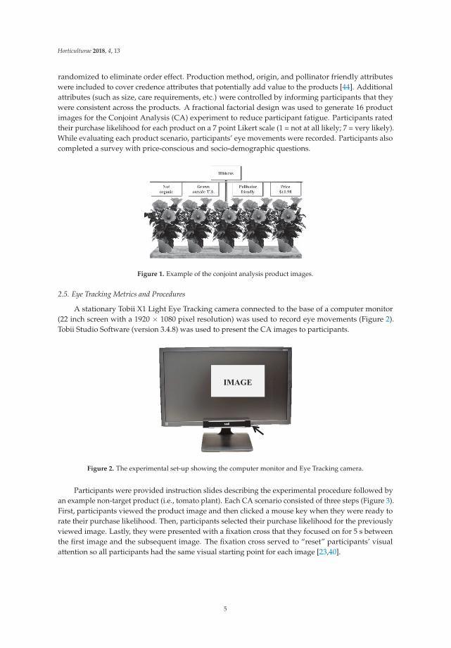
The Conjoint Analysis (CA) experiment was designed using ornamental landscape plants (i.e.,bedding plants, flowering annuals, and perennials) as the product, since they generated the most plantsales in Florida in 2013 [40]. Additionally, plants were selected as a product because they typically aresold with very little in-store signage and limited brand promotions [41]. Consequently, participants’preconceptions about the products are more limited than highly branded or promoted products.Several species of plants (petunias, pentas, and hibiscus) were included in the analysis to account fordifferences in individual preferences (Table 2). To simulate a common retail garden center display,five plants were presented on a bench, with additional attributes (i.e., price, production method, origin,and pollinator friendly attributes) being presented as above-plant signs (Figure 1). Previous studieshave successfully used this bench/attribute sign design to elicit consumers’ purchasing preferences forornamental plants [2,42,43].

Table 2. Attributes and attribute levels.

Attributes Attribute Levels Definition/Description

Plant type aHibiscus

PentaPetunia b

The type of plant in the scenario imageshown to participants.

Price a$10.98$12.98$14.98

Price per plant.

PollinatorPollinator friendly Indicates if the plant benefits pollinators.

No label b

Production method Certified organic Plants are certified as organically produced.

Organic production Plants are produced in an organic manner,but are not certified organic.

Not organic (conventional) b Plants are grown using conventionalproduction methods.

Origin In-state (Fresh from Florida) Plants are produced in Florida

Domestic (Grown in the U.S.) Plants are produced in the U.S.

Imported (Grown outside the U.S.) b Plants are imported from countries outsidethe U.S.

a Plant types and price points were selected based on products and prices at several retail outlets (i.e., big box stores,independent garden centers, etc.) in the study area. b Indicates base variables.

In this study, three price points ($10.98, $12.98, $14.98) were used based on prices of similarplants in higher end specialty garden centers, as well as lower price points from mass retailersand box stores in the study area (Table 2). Production methods included certified organic, organicproduction (but not certified), and conventional levels. Origin attributes included in-state, domestic,and imported levels. The pollinator friendly attribute was either labeled or not labeled. Sign order was

4


randomized to eliminate order effect. Production method, origin, and pollinator friendly attributeswere included to cover credence attributes that potentially add value to the products [44]. Additionalattributes (such as size, care requirements, etc.) were controlled by informing participants that theywere consistent across the products. A fractional factorial design was used to generate 16 productimages for the Conjoint Analysis (CA) experiment to reduce participant fatigue. Participants ratedtheir purchase likelihood for each product on a 7 point Likert scale (1 = not at all likely; 7 = very likely).While evaluating each product scenario, participants’ eye movements were recorded. Participants alsocompleted a survey with price-conscious and socio-demographic questions.

Figure 1. Example of the conjoint analysis product images.

2.5. Eye Tracking Metrics and Procedures

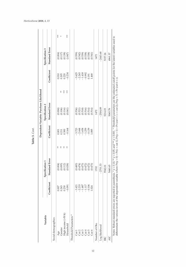
A stationary Tobii X1 Light Eye Tracking camera connected to the base of a computer monitor(22 inch screen with a 1920 × 1080 pixel resolution) was used to record eye movements (Figure 2).Tobii Studio Software (version 3.4.8) was used to present the CA images to participants.

Figure 2. The experimental set-up showing the computer monitor and Eye Tracking camera.

Participants were provided instruction slides describing the experimental procedure followed byan example non-target product (i.e., tomato plant). Each CA scenario consisted of three steps (Figure 3).First, participants viewed the product image and then clicked a mouse key when they were ready torate their purchase likelihood. Then, participants selected their purchase likelihood for the previouslyviewed image. Lastly, they were presented with a fixation cross that they focused on for 5 s betweenthe first image and the subsequent image. The fixation cross served to “reset” participants’ visualattention so all participants had the same visual starting point for each image [23,40].

5


Step

1. P

rodu

ct Im

age

Step

2. P

urch

ase

Like

lihoo

d Ra

ting

Step

3. F

ixat

ion

Cro

ss

Fig

ure

3.

The

thre

e-st

epex

peri

men

talp

roce

dure

used

for

the

16co

njoi

ntan

alys

issc

enar

ios.

6


After all participants had completed the experiment, areas of interest (AOI) were used to extractvisual attention measures from the product images. Each AOI corresponds to a specific visual ofinterest (i.e., the product image or an attribute sign; Figure 4). Researchers extracted participants’fixation count (FC) for each AOI. FC is the total number of eye fixations (when the eye stops andattends to the stimuli) within each AOI. FCs are considered a reliable indicator of participants’ visualattention to stimuli within each AOI [2,23].

Figure 4. Designated areas of interest (indicated by the dashed lines) around the product image andattribute signs.

2.6. Econometric Model

To investigate how price-conscious consumers may behave differently in term of purchasepatterns, we follow Long and Freese’s [45] ordered logit model and post-estimation proceduresto estimate predicted probabilities of participants’ purchase likelihood. As shown in Figure 3,the purchase likelihood was measured using a 7-point Likert scale question, with 1 indicating veryunlikely to purchase and 7 indicating very likely to purchase. The ordered logit model captures thenature that order of response matters. Let yi be the ordered rating scores of purchase likelihood,which is of interest to explain. yi is assumed to be generated by the underlying linear latent variablemodel:

y∗i = xiβ + εi (1)

where y* is varying from −∞ to ∞, i is the observation, and ε is a random error term. Our observedresponse categories (yi) are linked to the latent variable using the following subsequent measurementmodel:

yi =

⎧⎪⎪⎪⎪⎨⎪⎪⎪⎪⎩

12...

7

i fi f...

i f

κ0 = −∞ ≤ y∗i < κ1

κ1 ≤ y∗i < κ2...

κ6 ≤ y∗i < κ7 = ∞

(2)

where κ are thresholds that once crossed result in a category change. In the rest of the models, i issuppressed. Thus, the probability of observing y = j for given values of x is:

Pr(y = j|x) = Pr(κj−1 ≤ y∗ < κj

∣∣x) (3)

7


and j = 1 to J (purchase likelihood rating). Consequently, the predicted probability can be given as:

Pr(y = j|x) = F(κj − xβ

)− F(κj−1 − xβ

)(4)

where F indicates the cumulative distribution function of ε, and for ordered logit the ε is assumed tohave a logistic distribution with a mean of 0 and variance of π2/3.

The dependent variable (purchase likelihood) is a rating score (1 = very unlikely; 7 = very likely)and the key independent variables of interest are the price-consciousness indicator and the FCson the price sign. Other control variables include plant attributes (plant type, production method,origin) and individual socio-demographics, as well as visual data (fixation counts) on other non-priceproduct attributes.

3. Results and Discussion

Prior to regression analysis, we first compare price conscious consumers’ visual attention toprice versus non-price attitudes, which were measured by FCs. With a mean FC of 2.6, priceconscious consumers are typically less attentive to price than non-price attributes (compared toa mean FC of 3.3 across non-price attributes). The paired t-test statistic for each pair of price andnon-price attributes (including pollinator friendly, production method, and origin) comparison issignificant at 1% significant level except for when price and in-state attributes are compared. This resultcontradicts Hypothesis H1a that price conscious consumers would fixate more on price than non-priceattributes. Further, a direct comparison of price-conscious and non-price conscious consumers’ FCs isprovided in Figure 5. Overall, price conscious consumers spend less time fixating on the total image,products, prices, origins, certified organic, and conventional signs than the non-price conscious group,except for the organically produced sign. The mean FC for non-price conscious consumers is 2.7,which is slightly more than that of the price-conscious group (2.6). Nonetheless, the difference isnot statistically significant (pairwise t-test static is 1.20 with a p-value of 0.23). This result does notsupport Hypothesis H1b that price conscious consumers fixate more on price than non-price consciousconsumers. Although there is no significant difference in terms of visual attention on price betweenprice-conscious and non-price conscious groups, price conscious consumers tend to be more efficient(i.e., have fewer total fixations and fewer fixations on price and other attributes) than non-priceconscious consumers when determining their purchase likelihood. Since price conscious consumersvalue price over other attributes [2,12], this may reduce their visual consideration time on differentattributes because the attributes are less important than price. Alternatively, the price consciousconsumers may have been quicker decision makers due to having preexisting reference prices andprice cut-off values. Preexisting cut-off values streamlines the decision making process because if theproduct does not align with the reference prices, the product is eliminated from the choice set [46].

8


Figure 5. Mean Fixation Counts, by Price Consciousness. * indicates the mean difference between priceconscious and non-price-conscious consumers is significant (p < 0.05) based on pairwise t-test.

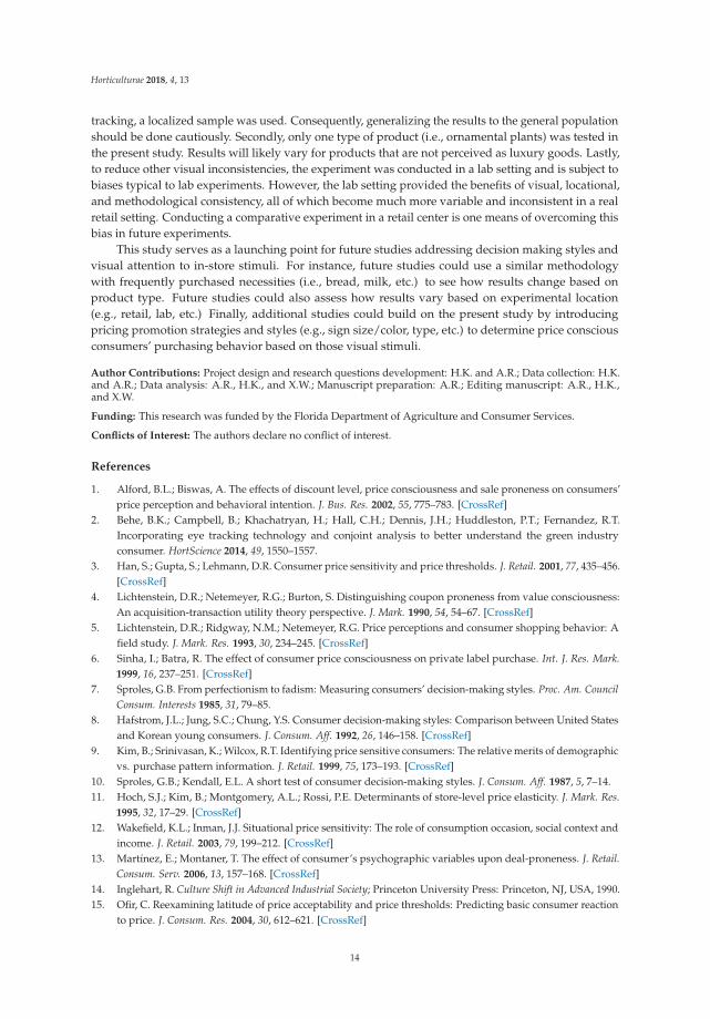
To fully explore price conscious consumers’ purchasing decisions and test Hypotheses H2a, H2b,and H3, three different specifications of the ordered logit model are estimated. Baseline Specification 1includes only the price-conscious indicator, plant attributes, and individual demographic information.Specification 2 and Specification 3 add visual attention variables (model 2) and interaction termsbetween price-conscious indicators to test H2a and H2b, and visual attention variables (model 3)to test H3, respectively. Recent studies have shown attention (i.e., visual attention) provides anadditional explanation for how consumers selectively process product information and is a crucialaspect that should be considered when analyzing individual choice behavior, including purchasingdecisions [24,29]. The interaction terms between the price-conscious indicator and visual attentionvariables, specifically, the interaction between the price conscious indicator and FCs on price (PC × FCprice), further distinguishes price conscious consumers from non-price conscious consumers to test H3.Indicated by the lower Bayesian Information Criterion (BIC) and Akaike Information Criterion (AIC)values (Table 3), Specification 2 and Specification 3 have largely improved the model fit and modelexplanation power by incorporating visual attention data.

Regression results (Table 3) from the ordered logit model indicate that price conscious consumersare significantly less likely to purchase plants in comparison with non-price conscious consumersregardless of the model specification, supporting Hypothesis H2a. The average marginal effect basedon Specification 1 indicates that a price conscious consumer, ceteris paribus, is 1.6 percentage points morelikely to rate themselves as “very unlikely” to purchase a plant, while 4.4 percentage points less likelyto rate themselves as “very likely” to purchase a plant. In addition, plant attributes (plant type, price,pollinator friendly, production method, and origin), respondents’ social-demographic characteristics,and visual attention variables all influence the purchase likelihood. Respondents are more likely topurchase hibiscus and pentas plants than petunia plants. As expected, price is negatively associatedwith purchase likelihood. Consistent with previous empirical evidence [47–50], we also find thatconsumers value products “being green” or sustainable. Particularly, the pollinator friendly attributeincreases consumers’ purchase intention. Respondents are also more likely to purchase certified organicor organically produced plants than conventionally produced plants. Regarding origin, in-state anddomestically grown plants are preferred to imported plants.

9


In terms of social-demographic characteristics, we find purchase likelihood increases with age.Male participants are more likely to purchase products than females as shown by the positive coefficientestimates across all specifications. Respondents with higher incomes are more likely to purchaseproducts than respondents with lower incomes. Conversely, having a larger household size discouragespurchase likelihood.

The visual attention data indicates there are statistically significant relationships between priceconsciousness, fixations, and purchase likelihood (Specification 2, Table 3). After controlling forconsumers’ visual attention, the negative impact of the price-conscious indicator on purchase likelihoodremains statistically significant. Consistent with price theory and existing empirical evidence (e.g.,Chen et al. [29]), increasing visual attention to the price sign discourages the likelihood of purchase,supporting Hypothesis H2b. Meanwhile, we find several positive relationships between consumers’visual attention to non-price attributes and their purchase likelihood. For example, more FCs onattribute signs, such as pollinator friendly, production method, and grown outside the United States,increases purchase likelihood. These results are in line with Van Loo et al. [23], finding that consumersfixate more on attributes that they value more and, thus, are more likely to purchase them.

10


Ta

ble

3.

Coe

ffici

ente

stim

ates

ofco

nsum

ers’

purc

hase

likel

ihoo

dof

orna

men

talh

orti

cult

ural

plan

tsfr

omth

eO

rder

edLo

gitR

egre

ssio

nM

odel

s.

Vari

ab

le

Dep

en

den

tV

ari

ab

le:

Pu

rch

ase

Lik

eli

ho

od

Sp

eci

fica

tio

n1

Sp

eci

fica

tio

n2

Sp

eci

fica

tio

n3

Co

effi

cien

tS

tan

dard

Err

or

Co

effi

cien

tS

tan

dard

Err

or

Co

effi

cien

tS

tan

dard

Err

or

Pric

e-co

nsci

ous

indi

cato

r(P

C)

−0.2

90(0

.106

)**

*−0

.251

(0.1

08)

**−0

.254

(0.1

14)

**

Plan

tatt

ribu

te

Hib

iscu

s0.

663

(0.1

16)

***

0.71

6(0

.120

)**

*0.

733

(0.1

21)

***

Pent

a0.

414

(0.1

10)

***

0.44

2(0

.114

)**

*0.

468

(0.1

12)

***

Petu

nia

Base

Base

Base

Pric

e−0

.175

(0.0

29)

***

−0.2

04(0

.030

)**

*−0

.208

(0.0

30)

***

Polli

nato

rfr

iend

ly0.

319

(0.0

94)

***

0.32

7(0

.097

)**

*0.

333

(0.0

95)

***

Cer

tifie

dor

gani

c0.

541

(0.1

15)

***

0.51

4(0

.118

)**

*0.

544

(0.1

20)

***

Org

anic

prod

ucti

on0.

722

(0.1

25)

***

0.69

9(0

.128

)**

*0.

7333

(0.1

28)

***

Con

vent

iona

lBa

seBa

seBa

seIn

-sta

te1.

061

(0.1

24)

***

1.15

6(0

.131

)**

*1.

222

(0.1

34)

***

Dom

esti

c0.

817

(0.1

23)

***

0.92

2(0

.128

)**

*0.

972

(0.1

31)

***

Impo

rtBa

seBa

seBa

se

Vis

ualA

tten

tion

Var

iabl

es

FC_p

rodu

ctim

age

0.02

5(0

.009

)**

*0.

053

(0.0

11)

***

FC_p

rice

−0.0

49(0

.006

)**

*−0

.045

(0.0

10)

***

FC_p

ollin

ator

frie

ndly

0.21

4(0

.070

)**

*0.

322

(0.0

86)

***

FC_c

erti

fied

orga

nic

0.20

8(0

.068

)**

*0.

367

(0.0

93)

***

FC_o

rgan

icpr

oduc

tion

−0.0

64(0

.033

)*

−0.0

30(0

.047

)FC

_con

vent

iona

l0.

159

(0.0

38)

***

0.16

8(0

.044

)**

*FC

_in-

stat

e−0

.033

(0.0

45)

−0.0

27(0

.053

)FC

_dom

esti

c0.

023

(0.0

48)

−0.1

80(0

.062

)**

*FC

_im

port

0.19

9(0

.034

)**

*0.

037

(0.0

47)

PCin

tera

ctin

gw

ith

Vis

ualA

tten

tion

PC×

FC_p

rodu

ctim

age

−0.1

43(0

.024

)**

*PC

×FC

_pri

ce−0

.411

(0.2

16)

*PC

×FC

_pol

linat

orfr

iend

ly−0

.780

(0.1

63)

***

PC×

FC_c

erti

fied

orga

nic

−0.0

42(0

.157

)PC

×FC

_org

anic

prod

ucti

on−0

.041

(0.0

82)

PC×

FC_c

onve

ntio

nal

−0.1

35(0

.114

)PC

×FC

_in-

stat

e−0

.007

(0.1

27)

PC×

FC_d

omes

tic

0.57

6(0

.107

)**

*PC

×FC

_im

port

0.61

2(0

.087

)**

*

11


Ta

ble

3.

Con

t.

Vari

ab

le

Dep

en

den

tV

ari

ab

le:

Pu

rch

ase

Lik

eli

ho

od

Sp

eci

fica

tio

n1

Sp

eci

fica

tio

n2

Sp

eci

fica

tio

n3

Co

effi

cien

tS

tan

dard

Err

or

Co

effi

cien

tS

tan

dard

Err

or

Co

effi

cien

tS

tan

dard

Err

or

Soci

al-d

emog

raph

ics

Age

0.00

7(0

.004

)**

0.00

1(0

.004

)0.

010

(0.0

04)

***

Gen

der

0.24

3(0

.095

)**

0.21

1(0

.106

)**

0.20

5(0

.117

)*

Hig

hin

com

e(>

50k)

0.23

0(0

.112

)**

0.30

0(0

.116

)**

*0.

220

(0.1

38)

Hou

seho

ld−0

.091

(0.0

38)

**−0

.164

(0.0

41)

***

−0.2

34()

.047

)**

*

Thr

esho

ldPa

ram

eter

sa

Cut

1−3

.421

(0.4

83)

−3.7

23(0

.536

)−3

.625

(0.5

59)

Cut

2−2

.233

(0.4

74)

−2.4

44(0

.521

)−2

.265

(0.5

42)

Cut

3−1

.487

(0.4

73)

−1.6

58(0

.518

)−1

.418

(0.5

39)

Cut

4−1

.117

(0.4

72)

−1.2

59(0

.516

)−0

.992

(0.5

38)

Cut

5−0

.106

(0.4

72)

−0.1

39(0

.514

)0.

191

(0.5

38)

Cut

61.

024

(0.4

73)

1.08

5(0

.514

)1.

468

(0.5

41)

Num

ber

ofO

bs.

1532

1472

1472

Log

likel

ihoo

d−2

701.

33−2

504.

89−2

443.

68

BIC

5542

.01

5214

.03

5157

.26

AIC

5440

.65

5065

.78

4961

.37

Not

es:R

obus

tsta

ndar

der

rors

are

repo

rted

inpa

rent

hesi

s.*

p<

0.10

;**

p<

0.05

;and

***

p<

0.00

1.a

Thre

shol

dpa

ram

eter

sar

eth

ees

timat

edcu

toff

poin

tsfo

rth

ela

tent

vari

able

sus

edto

diff

eren

tiat

eth

eva

riou

sle

vels

ofth

ede

pend

entv

aria

ble

whe

rePr

(y=

0)=

Pr(z

<cu

t1);

Pr(y

=1)

=Pr

(cut

1<

z<

cut2

);Pr

(y=

7)=

Pr(c

ut6

<z)

.

12


The complete relationship between price consciousness, visual consideration, and purchaselikelihood is captured by Specification 3 (Table 3). The impact of how increasing/decreasing visualattention to the price attribute may further affect price conscious consumers’ purchase likelihood,which is our primary interest, is jointly determined by the coefficients in front of FCs of price (FC_ price)and the interaction term between the price-conscious indicator and FCs of price (PC × FC_price).Both coefficients are negative and statistically significant, suggesting that increasing visual attentionon the price attribute will further reduce price conscious consumers’ purchase likelihood. This result isin support of Hypothesis 3, which states that price conscious consumers’ visual attention to price signswill inversely affect their purchase likelihood.

In addition, price conscious consumers who fixate on the product longer are less likely topurchase. Although FCs on the pollinator friendly attribute, in general, increases purchase likelihood,for price conscious consumers, more fixations corresponds with a decreased likelihood of purchase.The interaction terms between the price-conscious indicator and FCs on the three production methods(certified organic, organically produced, conventional) are not statistically significant, indicatingthat additional visual attention to production methods did not affect price conscious consumers’purchase decisions. In other words, visual attention does not differentiate the price-conscious groupof consumers from their counterparts in terms of preferences for production methods. Nonetheless,we do find, interestingly, that price conscious consumers with increased visual consideration of thedomestic and import origins are more likely to purchase the products. This result may be related toperceived price, since consumers are often willing to pay premiums for locally produced (‘in-state’)products [51,52]. Thus, domestic or import origins would likely be considered the less expensiveoptions by price conscious consumers. The visual attention results indicate that product attributes,which are perceived as “less expensive”, may improve price conscious consumers’ visual considerationand, ultimately, purchase likelihood.

4. Conclusions

Cumulatively, when examining price conscious consumers’ purchase likelihood and visualattention behavior, several patterns emerge. First, price conscious consumers typically pay lessvisual attention to price than other non-price information, such as plant type, production method,and origin. Compared to non-price conscious consumers, price conscious consumers spend less timeon the price attribute and less time evaluating the products (in general). This may indicate that they arefaster decision makers or have preconceived reference points for the various attributes that improvetheir speed of decision making. Second, for price conscious consumers, greater visual attention toproduct price information leads to a lesser purchase likelihood. As suggested by Chen et al. [29], pricesensitive consumers generally spend more time visually attending to the price attribute. Our resultsfurther refine their conclusion by demonstrating that longer fixations on the price information increasesprice conscious consumers’ price sensitivity and, thus, reduces their likelihood to buy. To the bestof our knowledge, this is the first study to explore how price conscious consumers perceive andreact to prices differently from non-price conscious consumers. The extent to which price consciousconsumers consider the price attribute of products when shopping is important from the consumerwelfare perspective.

A third pattern is that the relationship between visual attention to ‘less desirable’ and, potentially,‘less expensive’ options (e.g., domestic origins, import origins) improved price conscious consumers’purchase likelihood. This study does not delve into these motives, but they invite attention to potentialreasons behind price conscious consumers’ visual attention to various products/product attributesand suggests directions for future studies. Our results also have important implications for retailers.Retailers who are interested in targeting price conscious consumers and triggering them to buy shouldavoid promoting attributes that are perceived as more expensive (e.g., organic, local, etc.).

Despite providing interesting insights into price conscious consumers’ visual and purchasingbehavior, the present study does have several limitations that must be mentioned. First, to facilitate eye

13


tracking, a localized sample was used. Consequently, generalizing the results to the general populationshould be done cautiously. Secondly, only one type of product (i.e., ornamental plants) was tested inthe present study. Results will likely vary for products that are not perceived as luxury goods. Lastly,to reduce other visual inconsistencies, the experiment was conducted in a lab setting and is subject tobiases typical to lab experiments. However, the lab setting provided the benefits of visual, locational,and methodological consistency, all of which become much more variable and inconsistent in a realretail setting. Conducting a comparative experiment in a retail center is one means of overcoming thisbias in future experiments.

This study serves as a launching point for future studies addressing decision making styles andvisual attention to in-store stimuli. For instance, future studies could use a similar methodologywith frequently purchased necessities (i.e., bread, milk, etc.) to see how results change based onproduct type. Future studies could also assess how results vary based on experimental location(e.g., retail, lab, etc.) Finally, additional studies could build on the present study by introducingpricing promotion strategies and styles (e.g., sign size/color, type, etc.) to determine price consciousconsumers’ purchasing behavior based on those visual stimuli.

Author Contributions: Project design and research questions development: H.K. and A.R.; Data collection: H.K.and A.R.; Data analysis: A.R., H.K., and X.W.; Manuscript preparation: A.R.; Editing manuscript: A.R., H.K.,and X.W.

Funding: This research was funded by the Florida Department of Agriculture and Consumer Services.

Conflicts of Interest: The authors declare no conflict of interest.

References

1. Alford, B.L.; Biswas, A. The effects of discount level, price consciousness and sale proneness on consumers’price perception and behavioral intention. J. Bus. Res. 2002, 55, 775–783. [CrossRef]

2. Behe, B.K.; Campbell, B.; Khachatryan, H.; Hall, C.H.; Dennis, J.H.; Huddleston, P.T.; Fernandez, R.T.Incorporating eye tracking technology and conjoint analysis to better understand the green industryconsumer. HortScience 2014, 49, 1550–1557.

3. Han, S.; Gupta, S.; Lehmann, D.R. Consumer price sensitivity and price thresholds. J. Retail. 2001, 77, 435–456.[CrossRef]

4. Lichtenstein, D.R.; Netemeyer, R.G.; Burton, S. Distinguishing coupon proneness from value consciousness:An acquisition-transaction utility theory perspective. J. Mark. 1990, 54, 54–67. [CrossRef]

5. Lichtenstein, D.R.; Ridgway, N.M.; Netemeyer, R.G. Price perceptions and consumer shopping behavior: Afield study. J. Mark. Res. 1993, 30, 234–245. [CrossRef]

6. Sinha, I.; Batra, R. The effect of consumer price consciousness on private label purchase. Int. J. Res. Mark.1999, 16, 237–251. [CrossRef]

7. Sproles, G.B. From perfectionism to fadism: Measuring consumers’ decision-making styles. Proc. Am. CouncilConsum. Interests 1985, 31, 79–85.

8. Hafstrom, J.L.; Jung, S.C.; Chung, Y.S. Consumer decision-making styles: Comparison between United Statesand Korean young consumers. J. Consum. Aff. 1992, 26, 146–158. [CrossRef]

9. Kim, B.; Srinivasan, K.; Wilcox, R.T. Identifying price sensitive consumers: The relative merits of demographicvs. purchase pattern information. J. Retail. 1999, 75, 173–193. [CrossRef]

10. Sproles, G.B.; Kendall, E.L. A short test of consumer decision-making styles. J. Consum. Aff. 1987, 5, 7–14.11. Hoch, S.J.; Kim, B.; Montgomery, A.L.; Rossi, P.E. Determinants of store-level price elasticity. J. Mark. Res.

1995, 32, 17–29. [CrossRef]12. Wakefield, K.L.; Inman, J.J. Situational price sensitivity: The role of consumption occasion, social context and

income. J. Retail. 2003, 79, 199–212. [CrossRef]13. Martínez, E.; Montaner, T. The effect of consumer’s psychographic variables upon deal-proneness. J. Retail.

Consum. Serv. 2006, 13, 157–168. [CrossRef]14. Inglehart, R. Culture Shift in Advanced Industrial Society; Princeton University Press: Princeton, NJ, USA, 1990.15. Ofir, C. Reexamining latitude of price acceptability and price thresholds: Predicting basic consumer reaction

to price. J. Consum. Res. 2004, 30, 612–621. [CrossRef]

14


16. Elitzak, H. Food Cost Review, 1950–1997; Report No. 780, USDA Agricultural Economic Report; EconomicResearch Service: Washington, DC, USA, 1999.

17. Balcombe, K.; Bitzios, M.; Fraser, I.; Haddock-Fraser, J. Using attribute importance rankings within discretechoice experiments: An application to valuing bread attributes. J. Agric. Econ. 2014, 65, 446–462. [CrossRef]

18. Bundesen, C. A Theory of visual attention. Psychol. Rev. 1990, 97, 523–547. [CrossRef] [PubMed]19. Reutskaja, E.; Nagel, R.; Camerer, C.F.; Rangel, A. Search dynamics in consumer choice under time pressure:

An eye-tracking study. Am. Econ. Rev. 2011, 101, 900–926. [CrossRef]20. Arieli, A.; Ben-Ami, Y.; Rubinstein, A. Tracking decision makers under uncertainty. Am. Econ. J. Microecon.

2011, 3, 68–76. [CrossRef]21. Russo, J.E.; Leclerc, F. An eye-fixation analysis of choice processes for consumer nondurables. J. Consum. Res.

1994, 21, 274–290. [CrossRef]22. Van Loo, E.J.; Nayga, R.M.; Seo, H.S.; Verbeke, W. Visual Attribute Non-Attendance in a Food Choice Experiment:

Results From an Eye-Tracking Study; Agricultural and Applied Economics Association Annual Meeting:Minneapolis, MN, USA, 2014.

23. Van Loo, E.J.; Caputo, V.; Nayga, R.M.; Seo, H.S.; Zhang, B.; Verbeke, W. Sustainability labels on coffee:Consumer preferences, willingness-to-pay and visual attention to attributes. Ecol. Econ. 2015, 118, 215–225.[CrossRef]

24. Orquin, J.L.; Loose, S.M. Attention and choice: A review on eye movements in decision making. Acta Psychol.2013, 144, 190–206. [CrossRef] [PubMed]

25. Chandon, P.; Wansink, B.; Laurent, G. A benefit conguency framework of sales promotion effectiveness.J. Mark. 2000, 64, 65–81. [CrossRef]

26. Aschemann-Witzel, J.; Zielke, S. Can’t buy me green? A review of consumer perceptions of and behaviortoward the price of organic food. J. Consum. Aff. 2017, 51, 211–251. [CrossRef]

27. Magnusson, M.K.; Arvola, A.; Hursti, U.K.; Åberg, L.; Sjödén, P. Attitudes Towards Organic Foods AmongSwedish Consumers. Br. Food J. 2001, 103, 209–226. [CrossRef]

28. Grebitus, C.; Seitz, C. Relationship between attention and choice. In Proceedings of the European Associationof Agricultural Economists 2014 Congress “Agri-Food and Rural Innovations for Healthier Societies”,Ljubljana, Slovenia, 26–29 August 2014.

29. Chen, Y.; Caputo, V.; Nayga, R.M., Jr.; Scarpa, R.; Fazli, S. How visual attention affects choice outcomes: Aneye tracking study. In Proceedings of the 3rd International Winter Conference on Brain-Computer Interface,Sabuk, Korea, 12–14 January 2015.

30. Behe, B.K.; Bae, M.; Huddleston, P.T.; Sage, L. The effect of involvement on visual attention and productchoice. J. Retail. Consum. Serv. 2015, 24, 10–21. [CrossRef]

31. Huddleston, P.; Behe, B.K.; Minahan, S.; Fernandez, R.T. Seeking attention: An eye tracking study of in-storemerchandise displays. Int. J. Ret. Dist. Manag. 2015, 43, 561–574. [CrossRef]

32. Lichtenstein, D.R.; Bloch, P.H.; Black, W.C. Correlates of price acceptability. J. Consum. Res. 1988, 15, 243–252.[CrossRef]

33. Schimmenti, E.; Galati, A.; Borsellino, V.; Ievoli, C.; Lupi, C.; Tinervia, S. Behaviour of consumers ofconventional and organic flowers and ornamental plants in Italy. HortScience 2013, 41, 162–171.

34. Reisen, N.; Hoffrage, U.; Mast, F.W. Identifying decision strategies in a consumer choice situation.Judgm. Decis. Mak. 2008, 3, 641–658.

35. U.S. Census Bureau. State & County QuickFacts. 2014. Available online: http://quickfacts.census.gov/qfd/states/12000.html (accessed on 2 January 2018).

36. National Gardening Association. The Impact of Home and Community Gardening in America; Butterfield, B., Ed.;National Gardening Association, Inc.: South Burlington, VT, USA, 2009; pp. 1–17.

37. Kalyanaram, G.; Little, J.D.C. An empirical analysis of latitude of price Acceptance in consumer packagegoods. J. Consum. Res. 1994, 21, 408–418. [CrossRef]

38. Low, W.; Lee, J.; Cheng, S. The link betweeen customer satisfaction and price sensitivity: An investigation ofretailing industry in Taiwan. J. Retail. Consum. Serv. 2013, 20, 1–10. [CrossRef]

39. Stock, R.M. Can customer satisfaction decrease price sensitivity in business-to-business markets?J. Bus.-to-Bus. Mark. 2005, 12, 59–87. [CrossRef]

40. Hodges, A.W.; Khachatryan, H.; Hall, C.R.; Palma, M.A. Production and marketing practices and trade flowsin the United States Green Industry in 2013. J. Environ. Hortic. 2015, 33, 125–136.

15


41. Collart, A.J.; Palma, M.A.; Hall, C.R. Branding awareness and willingness-to-pay associated with the TexasSuperstar™ and Earth-Kind™ Brands in Texas. HortScience 2010, 45, 1226–1231.

42. Behe, B.K.; Zhao, J.; Sage, L.; Huddleston, P.T. Minahan, S. Display signs and involvement: The visual pathto purchase intention. Int. Rev. Retail. Dist. Consum. Res. 2013, 23, 189–203.

43. Behe, B.K.; Fernandez, R.T.; Huddleston, P.T.; Minahan, S.; Getter, K.L.; Sage, L.; Jones, A.M. Practical fielduse of eye-tracking devices for consumer research in the retail environment. HortTechnology 2013, 23, 517–524.

44. Hall, C.R.; Dickson, M.W. Economic, environmental, and health/well-being benefits associated with greenindustry products and services: A review. J. Environ. Hortic. 2011, 29, 96–103.

45. Long, J.S.; Freese, J. Regression Models for Categorical Dependent Variables Using STATA; A Stata PressPublication, StataCorp, LP: College Station, TX, USA, 2006.

46. Schiffman, L.G.; Kanuk, L.L. Consumer Behavior, 9th ed.; Prentice-Hall, Inc.: Upper Saddle River, NJ, USA,2007; pp. 177–178.

47. Dagher, G.; Itani, O. Factors influencing green purchasing behaviour: Empirical evidence from the Lebaneseconsumers. J. Consum. Behav. 2014, 113, 188–195. [CrossRef]

48. Khachatryan, H.; Rihn, A.L.; Campbell, B.; Yue, C.; Hall, C.; Behe, B.K. Visual attention to eco-labels predictsconsumer preferences for pollinator friendly plants. Sustainability 2017, 9, 1743. [CrossRef]

49. Miller, S.; Tait, P.; Saunders, C.; Dalziel, P.; Rutherford, P.; Abell, W. Estimation of consumer willingness-to-payfor social responsibility in fruit and vegetable products: A cross-country comparison using a choiceexperiment. J. Consum. Behav. 2017, 16, e13–e25. [CrossRef]

50. Yue, C.; Campbell, B.; Hall, C.R.; Behe, B.K.; Dennis, J.; Khachatryan, H. Consumer preference for sustainableattributes in plants: Evidence from experimenal auctions. Agribusiness 2016, 32, 222–235. [CrossRef]

51. Darby, K.; Batte, M.T.; Ernst, S.; Roe, B. Decomposing local: A conjoint analysis of locally produced foods.Am. J. Agric. Econ. 2008, 90, 476–486. [CrossRef]

52. Onozaka, Y.; McFadden, D.T. Does local labeling complement or compete with other sustainable labels?A conjoint analysis of direct and joint values for fresh produce claims. Am. J. Agric. Econ. 2011, 93, 693–706.[CrossRef]

© 2018 by the authors. Licensee MDPI, Basel, Switzerland. This article is an open accessarticle distributed under the terms and conditions of the Creative Commons Attribution(CC BY) license (http://creativecommons.org/licenses/by/4.0/).

16

horticulturae

Article

A Preliminary Assessment of HorticulturalPostharvest Market Loss in the Solomon Islands

Steven Jon Rees Underhill 1,2,*, Leeroy Joshua 2 and Yuchan Zhou 1

1 School of Science and Engineering ML41, University of the Sunshine Coast, Locked bag 4,Maroochydore DC, Queensland 4558, Australia; [email protected]

2 School of Natural Resources and Applied Sciences, Solomon Islands National University,PO BOX R113 Honiara, Solomon Islands; [email protected]


Received: 29 November 2018; Accepted: 4 January 2019; Published: 10 January 2019

Abstract: Honiara’s fresh horticultural markets are a critical component of the food distributionsystem in Guadalcanal, Solomon Islands. Most of the population that reside in Honiara are nowdependent on the municipal horticultural market and a network of smaller road-side markets tosource their fresh fruits and vegetables. Potentially poor postharvest supply chain practice could beleading to high levels of postharvest loss in Honiara markets, undermining domestic food security.This study reports on a preliminary assessment of postharvest horticultural market loss and associatedsupply chain logistics at the Honiara municipal market and five road-side markets on GuadalcanalIsland. Using vendor recall to quantify loss, we surveyed a total of 198 vendors between November2017 and March 2018. We found that postharvest loss in the Honiara municipal market was 7.9 to9.5%, and that road-side markets incurred 2.6 to 7.0% loss. Based on mean postharvest market lossand the incidence of individual vendor loss, Honiara’s road-side market system appears to be moreeffective in managing postharvest loss, compared to the municipal market. Postharvest loss waspoorly correlated to transport distance, possibly due to the inter-island and remote intra-island chainsavoiding high-perishable crops. Spatial mapping of postharvest loss highlighted a cohort of villages inthe western and southern parts of the main horticultural production region (i.e., eastern Guadalcanal)with atypically high levels of postharvest loss. The potential importance of market-operations,packaging type, and mode of transport on postharvest market loss, is further discussed.

Keywords: food security; postharvest; post-harvest; Pacific; food loss; municipal market; road-sidemarket; Honiara; Guadalcanal; Malaita

1. Introduction

Solomon Islands is a South Pacific archipelago consisting of six major islands and a further986 smaller islands, atolls and reefs. Around 84% of Solomon Islanders reside in rural villages and aredependent on subsistence-based agriculture and local fisheries [1,2]. In recent times, commercial foodsupply chains have become increasingly important in the Solomon Islands due to a combination of ruralto urban population drift [3,4], population growth [5,6], ongoing challenges associated with agriculturalproductivity [7], and the impacts of adverse weather events [1,2,8]. This trend is particularly acute inthe capital Honiara, with only 32% of the urban population having access to a home garden [6]. Mostof the population that resides in Honiara, are now dependent on the municipal horticultural marketand a network of smaller road-side markets to source their fresh fruits and vegetables.

Honiara’s horticultural markets not only provide important food security and human nutritionoutcomes [9,10], but create opportunities for local economic development and demonstrate a stronggender participation bias in favor of women market vendors [9,11]. The income generated from thesemarkets provides essential livelihood support for local squatter settlements in the “greater Honiara”



region [3] and are a primary source of income for many close proximity islands such as Savo Island [7]and possibly Florida Island. This combination of socio-economic, pro-gender engagement and foodsecurity and nutrition benefits, has led to an increased focus by donors on market-based interventionsin the Solomon Islands [12].

The need to improve the operational efficiency and effectiveness of the Honiara municipal markethave been widely recognized [2,11,12]. The Honiara municipal market is constrained by overcrowding,poor sanitation and concerns about vendor safety [12–14]. Most studies undertaken in support of theHoniara municipal markets have done so from a community resilience, gender and human securityperspective [3,4,7,11,15,16]. Its only recently that the underlying horticultural supply chains have beenexamined in any detail [7,11,16], providing a wider understanding of farm demographics, transportlogistics and vendor practice. What remains unclear, is how efficiently the Honiara markets and theirassociated supply chains operate in terms of postharvest horticultural loss. Unlike other South Pacificislands such as Fiji [17,18] and Samoa [19], there are no previous reported studies on postharvest marketloss in any of the markets in the Solomon Islands. With generic poor postharvest handling, potentiallyhigh-levels of postharvest loss in Honiara markets could be undermining domestic food security.

This study reports on a preliminary assessment of postharvest horticultural market loss andassociated supply chain logistics at the Honiara municipal market and five road-side markets onGuadalcanal Island. The inclusion of Honiara road-side markets in this study reflects an increasingrecognition of their importance in the overall food distribution system in Solomon Islands [15].This study is part of an ongoing longitudinal assessment of postharvest horticultural loss in Honiaramunicipal market and road-side markets (Guadalcanal Island), Auki municipal market (Malaita Island)and the Gizo municipal market (Ghizo Island).


2.1. Location

This study was undertaken at the Honiara municipal market and five road-side markets in theHoniara district, Guadalcanal Island and Solomon Islands (Figure 1A,B). The location of the road-sidemarkets assessed: Henderson, Fishing village, Lungga, King George VI and the White river, is shownin Figure 1B,C.

18


Figure 1. Map of the Solomon Islands. (A) Location of Guadalcanal Island (indicated in red) withinthe Solomon Islands archipelago (Map source: CartoGIS Services, College of Asia and the Pacific,The Australian National University, Australia, 2018); (B) map of Guadalcanal Island (red squareindicates the study site); (C) location of the Honiara municipal market and the five road-side markets,Guadalcanal Island (Map source: [email protected] Solomon Islands National Statistics Office, SolomonIslands, 2018).

2.2. Survey Design and Ethics Approval

Vendor surveys were undertaken in November 2017 and March 2018. Markets were concurrentlysurveyed, and involved a series of enumerators from the Solomon Islands National University (SINU)to support this study. The selection of vendors to be surveyed was randomised, but excluded thosevendors unable to identify where fruits and vegetables were grown (i.e., farm location) and thereforelikely to be involved in inter-market trade, those vendors selling value-added or non-perishableproducts, and those vendors unwilling to participate in the survey. The survey design was based onsemi-structured interview questions on harvesting and packaging practice, transport, market vendorpractice, and postharvest loss. Enumerators received prior training in the survey methodology andethics compliance.

A total of 198 vendors were assessed across all of the key Guadalcanal fruit and vegetable markets.This included 104 professional market vendors at the Honiara municipal market (42 vendors surveyedin November 2017 and an additional 62 vendors surveyed in March 2018). A further 94 road-sidemarket vendors (occasional traders) were also surveyed (42 road-side vendors surveyed in November2017 and 52 road-side vendors surveyed in March 2018). The survey was replicated across twosampling dates to partially account for potential differences in supply chain demographics andpostharvest handling practice due to crop seasonality.

Surveys involved a short semi-structured interview lasting 5–10 min, commonly undertaken inthe local language. All interviews were completed in compliance with the University of the SunshineCoast Human Research Ethics Approval (A16814).

19


2.3. Data Collected

Postharvest market loss was determined using vendor recall, consistent with other recent Pacificmarket loss studies [18,19]. This method excludes on-farm loss, does not include consumer waste nordoes it account for potential re-use of market loss for non-human consumption (i.e., product usedfor animal feed). For the purposes of this study, postharvest loss is defined as a fresh horticulturalproduct that was permanently removed from the chain due to being of an unsaleable quality andnot provided to others with the intent of human consumption [20]. Vendors were asked to quantifythe level of postharvest loss of the main horticultural products on-display at their individual vendorstalls. This allowed for postharvest loss and handling practice to be further segregated and analysedaccording to crop type.

Transport distance from the farm (village) to the market was determined using Google Earth Pro™Distance Calculator based on the most probable road transport route. Where the location of the villagecould not be directly identified, transport distance was calculated by cross referencing the map locationgiven by the vendor with the nearest village. Village locations were further validated in discussionswith the enumerators. For inter-island supply chains, transport distance was based on the most likelydirect ferry route. For the intra-island transport supply chains that involved a combination of boat androad transport, such as those from southern Guadalcanal, transport distance was calculated based ona boat transport route from the farm to the nearest village with continuous road access to Honiara,and the most probable road transport route thereafter.

Product was identified as either fruits, vegetables, or fruits and vegetables, based on generic(non-botanical) crop classification (i.e., tomato and similar crops were classified as vegetables).Semi-processed, processed and non-horticultural commodities were excluded from this study.

2.4. Statistical Analysis

Data analysis was undertaken using one-way analysis of variance (ANOVA). Analysis ofmarket vendor survey loss was undertaken using ANOVA followed by the Tukey–Kramer multiplecomparison test (with consideration for uneven vendor numbers between markets). The relationshipbetween market loss and transport distance was determined using a linear regression analysis.

3. Results

3.1. Postharvest Loss

Mean percent postharvest market loss at the Honiara municipal market was 9.5% in November2017 and 7.0% in March 2018 (Table 1). Mean percent postharvest loss for the road-side markets inGuadalcanal was 7.9% in November 2017 and 2.6% in March 2018. The level of postharvest loss wassignificantly higher in the Honiara municipal markets compared to the Honiara road-side market inthe March 2018 survey.

Table 1. Mean percent postharvest market loss for fresh fruits and vegetables sold in the Honiaramunicipal and road-side markets.

Market Type and LocationMean Percent

Postharvest Loss(November 2017)

Mean PercentPostharvest Loss

(March 2018)

Vendor with NoPostharvest Loss (%)

Honiara municipal market 9.5 z a w 7.0 x a 19.2Honiara road-side markets 7.9 z a 2.6 y b 44.7

Data relates to all fruits and vegetables combined. z n = 42. x n = 62. y n = 52. w Values followed by the same letterare not statistically different at p < 0.05 based on Tukey-Kramer test.

The frequency of postharvest loss differed between the municipal and road-side markets (Table 1).In the municipal market, most vendors experienced some level of postharvest loss, with only 19.2% of

20


vendor surveyed indicating no loss (Table 1). In contrast, nearly half of the road-side vendors (44.7%)reported no postharvest loss. When road-side market vendors incurred postharvest loss, the amountof loss tended be high (often 20 to 25% loss—data not shown).

Postharvest loss for fruits was 7% to 7.6% in the municipal market and 3% to 5.2% in road-sidemarkets (Table 2). In comparison, postharvest loss for vegetables tended to be more variable, 1.8 to12.7%, with significantly higher postharvest loss in municipal market in the November survey (Table 2).Low, but not significant, vegetable postharvest loss observed in road-side markets in the March surveywas due to fewer vendors reporting atypically high postharvest loss (data not shown).

Table 2. Mean percent postharvest market loss for fresh fruits and vegetables z sold in the Honiaramunicipal and road-side markets.

Market Type andLocation

Mean Percent PostharvestLoss (November 2017)

Mean Percent PostharvestLoss (March 2018)

Fruit Vegetable y Fruit Vegetable y

Honiara municipal market 7.0 efgh x 12.7 abcde 7.6 defgh 8.1 cdefghHoniara road-side markets 5.2 fgh 11.6 bcdef 3.0 gh 1.8 h

z Postharvest loss data relates to fresh fruits and vegetables but excludes all other food categories includingsemi-processed and cooked product. y Crops were defined as vegetables based on a commercial rather than botanicalclassification (i.e., tomato identified as a vegetable crop). X Values followed by the same letter within columns androws for individual market survey dates are not statistically different at p < 0.05 based on Tukey–Kramer test.

The portion of fruits to vegetables being sold differed during the two survey dates, possiblyreflecting seasonal supply. In November, 44% of vendors were selling fruits and 56% selling vegetables,whereas in the March survey 30% of vendors were selling fruits and 70% vegetables (data not shown).

Mean postharvest loss for inter-island and intra-island supply chains supplying the Honiaramunicipal market (November 2017 and March 2018 combined results) is shown in Table 3. Whileinter-island chains appear to have slightly higher loss, this trend could not be statistically assessed dueto the limited number of inter-chains included in the survey.

Table 3. Mean percent postharvest market loss for intra-island and inter-island located farms supplyingthe Honiara municipal market.

Supply Chains Mean Percent Postharvest

Guadalcanal Island to Honiara (intra-Island) 8.1 z

Malaita Island to Honiara 16.7 y

Savo Island to Honiara 11.2 x

Nggela Island to Honiara 16.3 w

Z n = 90 y n = 3; x n = 4; w n = 2.

3.2. Supply Chain Logistics

Fresh fruits and vegetables sold in the Honiara municipal market were primarily sourced fromfarms located to the east of Honiara, and to a lesser extent, villages on the north–west of GuadalcanalIsland (Figure 2). Products sourced from farms located to the west of Honiara were more commonduring the November sampling period. Few farms located in the southern parts of Guadalcanalsupply the Honiara municipal market. A small percentage of Honiara municipal market vendors(8.7%) were sourcing produce from Malaita, Gizo and Savo Islands (Figure 2). Inter-island sourcedproducts were only observed in the Honiara municipal market, with the road-side markets tending tosource locally-grown products.

21


Figure 2. The locations (green marked areas) of farms supplying the Honiara municipal and road-sidemarkets during the survey period (November 2017 and March 2018 data combined). (Source: Basemap: [email protected] Solomon Islands National Statistics Office, Solomon Islands, 2018). Note locationof farms are not GIS positioned.

Horticulture transport logistics into the Honiara municipal market were relatively short,with products travelling 40 to 47 km (Table 4). In comparison, products supplying the road-sidemarkets travelled 19 to 27 km, almost half the distance. Some of this disparity can be attributed to theinclusion of inter-island supply chains into the Honiara municipal market. When the median transportdistances are considered, the transport distance between farms and municipal markets or road-sidemarkets were relatively similar in the November 2017 survey. In the March 2018 survey, mean transportsupply distance for road-side markets was 17.1 km (Table 4). This reduction in transport distanceimplies vendors are able to source more products locally, and may explain the lower incidence ofpostharvest loss observed in road-side markets during this time (Table 2).

Table 4. Transport distance from the farm to the municipal or road-side markets.

Market Type and Location Mean Transport Distance (km) Median Transport Distance (km)

Honiara municipal market (November 2017) 40.0 32.9Honiara road-side markets (November 2017) 26.9 28.0 z

Honiara municipal market (March 2018) 46.6 38.1Honiara road-side markets (March 2018) 18.6 17.1 z

z Road-side market data represents data sourced from the Henderson, Fishing Village, Lungga, King George VI andWhite river road-side markets.

The mean transport distance for the individual road-side market network varied depending onthe market location and the survey date (Table 5). Products sold at the Lungga and King George VImarkets tended to be sourced from smallholder farmers located in close proximity to these markets(1 to 2 km away). Whereas products supplying the larger White river and Fishing village marketstravelled 24 to 37 km. The comparatively shorter transport distances for the White river noted in theNovember survey and for the Henderson and Fishing village markets in the March survey are thoughtto reflect possible crop seasonal variability in the supply chains.

22


Table 5. Mean transport distance from the farm to the individual road-side markets.

Market Type and LocationMean Transport Distance (km)

(November 2017)Mean Transport Distance (km)

(March 2018)

Henderson 40.7 14.3Lungga and King George VI

(combined) 2.16 1.35

Fishing Village 37.7 26.8White river 24.3 30.9

The most common mode of transport used by farmer/vendors to transport product to theHoniara markets (municipal and road-side) was by truck (Table 6). Truck-based transport systemswere associated with farms located in more remote intra-island locations, with a mean travel distanceof 37 km. However, there was considerable variability in transport distances involving trucks, with theshortest recorded transport distance being 6.2 km and the furthest being 64.8 km.

Table 6. Mode of transport used and mean transport distance for all markets and all survey dates.

Mode of TransportMean Transport Distance

(km)Percent of Farmers/Vendors Using Specific

Mode of Transport (%)

Ferry/boat 88.9 a z 6.7Truck 37.0 bcde 54.2Car 25.2 cde 4.5

Minivan/public bus 20.5 de 14.5Taxi 8.5 e 13.4Walk 1.3 f 6.7

z Values followed by the same letter are not statistically different at p < 0.05 based on Tukey–Kramer test.

Mean transport distance involving cars or minivans/public buses was 20 to 25 km (Table 6).There was also considerable variability in the transport distance by car—ranging from 3.7 to 44.7 km,and transport distance by minivan/public bus—ranging from 0.5 to 41.2 km.

Transport by taxi was limited to farmers located relatively close to the market, with a meantransport distance of 8.5 km (Table 6).

3.3. Potential Contributions to Postharvest Loss

There was a weak correlation between transport distance and postharvest loss (Figure 3). Farmswith very high levels of postharvest loss (>30% loss) were primarily located within 50 km of themarkets. Conversely, most supply chains with a transport distance of 100 to 200 km had less than10% loss.

The location of farms with moderate (10 to 19%) to very high levels (>30%) of postharvesthorticultural loss are shown in Figure 4. Elevated postharvest loss was more prevalent in supplychains sourcing products from the far eastern part of the main production center (see Figures 2 and 4).There were multiple supply chains sourcing products from Tutumu, Tenaru, Vatukukau, Ruavatu,Siara, Binu, Aola, Tasimboko, Dadai villages on Guadalcanal Island, and Matakwara and Buma villageson Malaita Island with moderate to very high levels of postharvest loss. While there are relatively fewfarms located on the southern and far western parts of Guadalcanal supplying the Honiara markets(Figure 2), none of these had elevated postharvest loss (Figure 4).

23


Figure 3. A linear regression analysis of percent postharvest loss verses transport distance for allvendors, markets and survey dates (n = 346). R2 = 0.2503.

Figure 4. The locations of farms supplying the Honiara municipal or road-side markets with elevatedlevels of postharvest loss. (Source: Base map: [email protected] Solomon Islands National StatisticsOffice, Solomon Islands, 2018). Note farm locations are not GIS positioned.

The type of products being sourced by market vendors differed depending on farm location(Figure 5). Inter-island supply chains and those chains sourcing from the remote farms on GuadalcanalIsland were less likely to include vegetables. Vendors instead tended to source vegetables fromcloser proximity intra-island located farms, especially those in the “greater Honiara” region andnorth-eastern Guadalcanal.

The most commonly sourced product from remote farms (>50 km) was watermelon, green bananaand English cabbage (Table 7). Highly-perishable crops sourced from remote farms on Guadalcanaltended to be higher-value Asian leafy vegetables such as Pak choi and Choy sum (Table 7). Meanpostharvest loss for these chains was 13.2% with half the consignments incurring ≥20% loss (datanot shown).

24


Figure 5. The commodity composition (vegetables to fruits ratio) of consignments sourced from intraverses inter-island located farms. (A) Intra-island supply chains (Guadalcanal) into the Honiara market;(B) Inter-island supply chains into the Honiara market. Data is based on number of consignments,rather than consignment volume or weight.

Table 7. The most common commodities being sourced by vendors at the Honiara municipal marketfrom remote located farms (>50 km from farm to market).

Commodity Rank Order

Watermelon 13.3%Green banana, English cabbage 11%

Pak choi, pineapple 8.9%Cucumber, shallots 6.7%Choy sum, citrus 4.4%

A wide range of different packaging types were observed in the markets (Table 8). Large sacks(≥40 kg) were the most common type of packaging, especially for leafy indigenous vegetables. Highervalue crops such as tomato and Asian vegetables tended to be limited to smaller (<20 kg) packingunits. Postharvest loss was highest in very large packing units (Table 8).

Table 8. Mean postharvest loss based on packaging type.

Package Type Mean Postharvest Loss (%)Percentage of Supply Chains

Using Packaging Type y

Very large sacks (>100 kg net weight) 10.9 a z 8.4%Large sacks (approx. 40 kg) 4.9 b 34.0%

Medium sacks (20 kg) 5.5 ab 17.9%z Values followed by the same letter are not statistically different at p < 0.05 based on Tukey–Kramer test. y Vendorsalso used a range of other packaging options: plastic trays (14.2% of vendors), small plastic bags (5–10 kg) (10.5%),plastic crates (1.5%), plastic buckets (3%), steel basins (8.4%), locally woven baskets (1.5%) and nil packaging (1.5%).

4. Discussion

Horticultural postharvest loss in the Honiara municipal market was 7.9 to 9.5%. In comparison,postharvest loss in the Honiara road-side markets tended to be lower (2.6 to 7.0%) but more variable.This level of loss was consistent with other South Pacific municipal markets, with Reference [19]reporting a 6.2% loss in the central municipal market in Samoa. Most municipal market vendors inHoniara experienced some level of postharvest loss, whereas road-side market vendor loss tendedto be less common. Based on mean postharvest market loss and the incidence of individual vendorloss, Honiara’s road-side market system appears to be more effective in minimising postharvest loss,compared to the municipal market.

25


The potential contributors to postharvest market loss in Guadalcanal markets and reasons forreduced loss in the road-side markets are likely to be multifaceted. Diverse market participation(commercial-scale farmers through to semi-subsistence farm surplus), poor road infrastructure, the lackof a cool chain, limited or poor packaging, and inadequate market storage facilities needs to balanceagainst potential supply chain practices that seek to mitigate or lessen potentially elevated postharvestloss. While the contributors to generic postharvest loss in horticultural markets have been widelyreported [19,21–24], the inclusion of possible vendor or farmer strategies to reduce this loss areoften overlooked.

Intuitively, it would be logical to assume that transport distance would have a significant effect onthe level of postharvest loss seen in the market, consistent with the findings in other postharvest supplychain studies [24,25]. While inter-island supply chains appear to have higher levels of postharvest losscompared to intra-island chains, we found that postharvest loss was poorly correlated to transportdistance. Farms with very high levels of postharvest loss (>30% loss) tend to be located within 50 kmof the markets, most supply chains with a transport distance of greater than 100 km have less than10% loss, and loss associated with very remote intra-island supply routes was similarly less than 10%.These observations would suggest that the distance horticultural produce needs to travel from thefarm to market is not a good indicator of potential market postharvest loss in Guadalcanal.

The type of crops sourced from inter-island and remote intra-island farms and their associatedsupply chain practice may provide some insight into the disconnect between transport distanceand postharvest loss. Most inter-island supply chains included in this study were dominated bysemi-perishable crops such as watermelon, pineapple and citrus. Such crops are often considered tobe more tolerant of challenging transport logistics and potentially prolonged market storage. In themore remote Malaita to Guadalcanal inter-island supply chains, the product was sourced from twofruit production centers, watermelons from Buma and pineapples from Bina. These chains involvedcommercial-scale farms with relatively predictable transport logistics, with resultant postharvestloss being relatively low (<5%). Georgeou et al. [11] reported that the most commonly traded cropsfrom Savo and Nggela Islands into the Honiara markets were fruits, nuts and root crops. In remoteintra-island chains, such as products sourced from Mbalo on the far south-eastern part of Guadalcanaland Tangarare on the far south eastern part of Guadalcanal, there was a similar dominance ofsemi-perishable crops such as watermelon and citrus. While this might simply reflect local agronomicproduction conditions favouring certain crops, it is also possible that there is deliberate strategy byfarmers supplying the Honiara market to avoid highly perishable cash crops if the associated transportlogistic is likely to incur high-levels of postharvest loss.

Vegetable supply chains still represented a significant portion of the overall inter-island tradeinto Honiara. A recent study of the Savo to Honiara market supply chains [16] reported not onlysemi-perishable crops but also highly perishable leafy vegetables being traded. Savo farmers indicatedhigh levels of postharvest loss due to in-transit damage and delays in accessing transport [16], eventhough Savo Island is only about 35 km from Honiara. The presence of inter-island trade of perishablevegetable crops in spite of high-levels of postharvest loss is interesting. Georgeou et al. [16] reportedthat much of the trade from Savo Island into the Honiara municipal market was due to opportunisticmarket participation due to surplus local production [16]. Faced with possibly few alternative localmarket opportunities on Savo Island, potentially high postharvest loss does not appear to disincentivisemarket participation.

When intra-island vendor loss was analysed in terms of where produce was grown, we found thatthere was a cohort of villages in the western and southern parts of the main horticultural production(which is located in eastern Guadalcanal) which were consistently associated with atypically highlevels of postharvest loss. This result might reflect the type of crops grown in these locations,with Reference [11] reporting that most of the perishable leafy vegetables sold in the Honiara municipalmarket were sourced from farms located in north-eastern Guadalcanal. An alternative or additionalpossibility is a lack of reliable commercial transport options in these villages, or generic poor harvesting

26


and handling practice. Further studies are required to better understand on-farm postharvest practiceand supply chain logistics within these villages. Spatial mapping of high-loss postharvest chains hasnot been previously reported in the South Pacific, and provides useful information in terms of helpingto better target possible future technical farmer assistance and supply chain remediation.

Supply chain modes of transport associated with Honiara’s markets reflect the diversity ofagronomic production systems, from the commercial-scale through to semi-subsistent trade farmsurplus. The most common form of transport was open trucks, consistent with the findings reportedby Reference [11]. Nearly all of the supply chains sourcing products from eastern Guadalcanal weredependant on trucks, possibly reflecting the volume of trade, poor road conditions and some levelof local transport coordination. In Samoa and Vanuatu, where there is a relatively well maintainedroad-network and small production volumes, public buses, minivans and private vehicles are morecommonly used [19]. While the mode of transport is interesting, the specific postharvest transportconditions need to be better understood. How crops are loaded and the load configuration withinthe truck, the volume being transported, other possible items being co-transported can also havea significant influence on postharvest loss. More work is required to better understand transportlogistics especially between eastern Guadalcanal and the Honiara markets as a possible contributor topostharvest loss.

A range of packing types were used by farmers, the most common of which was 40 kg of wovensacks. Given the large diversity of crops and packaging options, only a superficial assessment of theimplication of packaging type on loss could be undertaken. As anticipated, very large agricultural sacks(>100 kg) used transport traditional leafy vegetables incurred significantly high levels of postharvestloss compared to smaller sizes of the same packaging type. Most heavy produce (such as pineapples,watermelon) were transported loose (no packaging). In the case of pineapples, the product was oftentied into bundles of up to 40 fruit and carried using wooden poles. Plastic crates were rarely observed.Plastic buckets and steel trays were used for crops prone to damage during transport (such as tomatoand papaya). The packing options used by farmers and vendors is thought to simply reflect the typeof packaging readily available, with Reference [23] noting that vendors in Malaita Island were awareof the adverse implication of poor packaging.

Comparatively low postharvest loss (4 to 5%) associated with a commonly used form of packaging(i.e., woven sacks ≤40 kg) would suggest that while packing is far from ideal, for most farmers packinghad little effect on resultant postharvest loss. However, damage associated with poor packaging can belatent and, therefore, not immediately evident when product arrivals at the market. Georgeou et al. [11]reported that product in the Honiara municipal market is commonly sold with 1/2 to 1 day or arrivingat the market. It is possible that the potential full implications of poor packaging may be somewhatnegated due to rapid market-throughput.

How efficiently the market-to-consumer food system operates directly influences postharvestsupply chain loss. Noting high tropical ambient conditions, prolonged market storage has beenreported to significantly elevate postharvest loss in other Pacific horticultural markets [19].The observation by Reference [11], that most vendors in the Honiara municipal market sell theirproduce within 1/2 to 1 day is therefore significant. Honiara’s road-side markets are likely to experienceeven more rapid product throughput due to fewer vendors and smaller volumes of product being sold,reducing vendor competition, and road-side markets located close to the resident’s areas increasingpotential consumer accessibility. In comparison, a product traded through the municipal market inSamoa is often stored for 2 to 3 days before it can be sold [19]. In Samoa, the benefits of comparativelygood on-farm postharvest handling practice and shorter transport distances are being underminedby prolonged market storage [19]. In the Honiara markets, rapid market throughput of a perishableproduct is thought to be an important factor in avoiding potentially higher-levels of postharvest lossdue to poor on-farm and transport practice. Fast on-selling by vendors in the Honiara municipalmarket is not the result of a better designed market infrastructure. Instead, high market vendor fees,over-crowding, poor market storage conditions, and significant concerns over vendor safety and

27


hygiene create tangible incentives for Honiara vendors to sell their produce as quickly as possible.Further studies are required to better understand road-side market trading practices and whetherthis further contributes to slightly lower postharvest loss in these markets. The implications ofcurrent vendor practice on postharvest loss at the consumer-end of the value chain also warrantsfurther investigation.

One variable that needs to be considered when interpreting market survey data in this studyis the potential for inter-market trade (particularly between the Honiara municipal market and thevarious road-side markets). Georgeou et al. [11] reported that approximately 30% of consumers atthe Honiara market were on-selling products in other markets. In this study, we sought to excludevendors who had sourced products from other markets from the survey, however, 2.6% of marketvendors surveyed were unable to identify the farm location where the product was sourced. However,given that Reference [11] further highlighted ongoing tension between farmer vendors and re-sellers,suggesting that re-sellers may not self-identify when surveyed, we cannot exclude the possibility ofsome level of data error based on vendors providing deliberately inaccurate survey responses.

5. Conclusions

Horticultural postharvest loss in the Honiara municipal market is consistent with the level ofloss in the Apia municipal market, Samoa. Guadalcanal’s road-side vendors appear to experienceless postharvest loss than vendors in the municipal market; however, the reasons for this are stillunclear. The level of loss observed in Guadalcanal’s postharvest markets is thought to be due toa combination of poor packaging, the type of crops being sold and possible opportunistic marketparticipation associated with trade farm surplus. While the types of transport used by smallholderfarmers were documented, their contribution to postharvest loss is unclear. We believe that potentiallyhigher market loss is being mitigated by market vendor practice. Rapid market throughput-associatedfast on-selling of the product reduces the time a product requires to be stored in the market. Farmerswith potentially challenging transport supply chain logistics, which are likely to incur high postharvestloss, appear to be avoiding highly perishable crops in favor of semi-perishable fruit and starchyroot crops. The observation of a series of farms toward the western and southern margins of themain production center with atypically high levels of postharvest loss warrants further investigation.Similarly, further work is required to better understand on-farm harvest and postharvest practices andpossible elevated loss at the consumer-end of the chain.

Author Contributions: Conceptualization, S.J.R.U. and L.J.; methodology, S.J.R.U. and L.J.; investigation, L.J.;statistical analysis, Y.Z.; writing—original draft preparation, L.J. and S.J.R.U.; writing—review and editing, S.J.R.U.,L.J. and Y.Z.; supervision, S.J.R.U.

Funding: This research was funded by the Food and Agriculture Organisation of the United Nations (FAO)grant number LoA SAP 2017/16 “Policy measures for the reduction of food loss/waste along fruit and vegetablevalue chains”.

Acknowledgments: We would like to express our sincere appreciation for the invaluable assistance and supportprovided by Michael Ho’ota and Selson John Ulasi (Ministry of Agriculture and Livestock, Solomon Islands),Nichol Nonga (FAO), Peter Iro (Solomon Islands National), and the Late Tim Martyn (FAO). We would also liketo acknowledge students from the Solomon Islands National University who assisted in data collection and thenumerous Solomon Island road-side and municipal market vendors and small-holder farmers, who providedtheir time and input in support of this study.

Conflicts of Interest: The authors declare no conflict of interest. The funders had no role in the design of thestudy; in the collection, analyses, or interpretation of data; in the writing of the manuscript, or in the decision topublish the results.

References

1. Schwarz, A.M.; Béné, C.; Bennett, G.; Boso, D.; Hilly, Z.; Paul, C.; Posala, R.; Sibiti, S.; Andrew, N. Vulnerabilityand resilience of remote rural communities to shocks and global changes: Empirical analysis from SolomonIslands. Glob. Environ. Chang. 2011, 21, 1128–1140. [CrossRef]

28


2. Evan, B.R. Solomon Islands Smallholder Agricultural Study: Literature Review—A Brief National Assessment of theAgricultural Sector; Australian Agency for International Development: Canberra, Australia, 2006; Volume 5,pp. 1–48, ISBN 1 920861 505.6.

3. Keen, M.; Kiddle, L. Priced out of the Market: Informal Settlements in Honiara, Solomon Islands; Department ofPacific Affairs: Canberra, Australia, 2016; p. 2.

4. Maebuta, H.; Maebuta, J. Generating livelihoods: A study of urban squatter settlements in Solomon Islands.Pac. Econ. Bull. 2009, 24, 119–129.

5. Solomon Islands National Statistical Office. Population Projected Population by Province 2010–2050.Statistics. Available online: http://www.statistics.gov.sb/statistics/social-statistics/population (accessed on14 September 2018).

6. Solomon Islands National Statistical Office. Solomon Islands 2012/13 Household Income and ExpenditureSurvey Provincial Analytical Report (Volume 2). Available online: http://www.statistics.gov.sb/statistics/demographic-statistics/household-income-and-expenditure-surveys (accessed on 14 September 2018).

7. Georgeou, N.; Hawksley, C.; Ride, A.; Kii, M.; Turasi, W. Human Security and Livelihoods in Savo Island, SolomonIslands: Engaging with the Market Economy: A Report for Honiara City Council; University of WollongongResearch Online: Sydney, Australia, 2015; pp. 1–31.

8. Anon. Solomon Islands Agriculture and Livestock Sector Policy 2015–2019. Available online: https://pafpnet.spc.int/images/articles/policy-bank/solomon/Solomons-Islands-NALSP_Final%20Draft_151118.pdf(accessed on 12 September 2018).

9. Andersen, A.B.; Thilsted, S.H.; Schwarz, A.M. CGIAR Research Program on Aquatic Agricultural Systems;Working Paper AAS-2013-06; Food and Nutrition Security in Solomon Islands: Penang, Malaysia, 2013.Available online: http://aquaticcommons.org/id/eprint/11081 (accessed on 12 September 2018).

10. Solomon Islands National Statistical Office. Solomon Islands Demographic and Health Survey 2006–2007;Secretariat of the Pacific Community: Noumea, New Caledonia, 2009; pp. 159–300.

11. Georgeou, N.; Hawksley, C.; Monks, J. Food security in Solomon Islands: Preliminary results from a surveyof the Honiara Central Market. Pac. Dyn. 2018, 2, 53–70.

12. DFAT. Solomon Islands Markets for Change. Available online: https://dfat.gov.au/about-us/publications/Documents/solomon-islands-markets-for-change-proposed-project-document.pdf (accessedon 14 September 2018).

13. FAO. Food and Nutrition Security Impact, Resilience, Sustainability and Transformation. Available online:http://www.fao.org/europeanunion/eu-projects/first/en/ (accessed on 14 September 2018).

14. DFAT. Aid Programme Performance Report 2016–2017—Solomon Islands. Available online:https://dfat.gov.au/about-us/publications/Documents/solomon-islands-appr-2016-17.pdf (accessed on14 September 2018).

15. Keen, M.; Ride, A. Markets Matter: Enhancing Livelihoods and Localities; Department of Pacific Affairs: Canberra,Australia, 2016; p. 2.

16. Georgeou, N.; Hawksley, C. Challenges for Sustainable Communities in Solomon Islands: Food Production,Market Sale and Livelihoods on Savo Island. J. Multidiscip. Int. Stud. 2017, 14, 67–86. [CrossRef]

17. Underhill, S.J.R.; Kumar, S. Postharvest handling of tropical fruit in the South Pacific. Fiji Agric. J. 2017,57, 19–26.

18. Underhill, S.J.R.; Kumar, S. Quantifying postharvest losses along a commercial tomato supply chain in Fiji.J. Appl. Hortic. 2015, 17, 199–204.

19. Underhill, S.J.R.; Zhou, Y.; Sherzad, S.; Singh-Peterson, L.; Tagoai, S.M. Horticultural postharvest loss inmunicipal fruit and vegetable markets in Samoa. Food Secur. 2017, 9, 1373–1383. [CrossRef]

20. Food Loss and Waste Protocol. Food Loss and Waste Accounting and Reporting Standard. Available online:http://www.wri.org/sites/default/files/FLW_Standard_final_2016.pdf (accessed on 16 December 2018).

21. Mashau, M.E.; Moyane, J.N.; Jideani, I.A. Assessment of post harvest losses of fruits at Tshakhuma fruitmarket in Limpopo Province, South Africa. Afr. J. Agric. Res. 2012, 7, 4145–4150. [CrossRef]

22. Masum, M.M.I.; Islam, S.M.M.; Islam, M.S.; Kabir, M.H. Estimation of loss due to post harvest diseases ofpotato in markets of different districts in Bangladesh. Afr. J. Biotechol. 2011, 10, 11892–118902.

23. Kumar, D.K.; Basavaraja, H.; Mahajanshetti, S.B. An economic analysis of post-harvest losses in vegetablesin Karnataka. Ind. J. Agric. Econ. 2006, 61, 134–146.

29


24. Kasso, M.; Bekele, A. Post-harvest loss and quality deterioration of horticultural crops in Dire Dawa Region,Ethiopia. J. Saudi Soc. Agric. Sci. 2016, 17, 88–96. [CrossRef]

25. Gangwar, L.S.; Singh, D.; Singh, D.B. Estimation of Post-Harvest Losses in Kinnow Mandarin in PunjabUsing a Modified Formula. Agric. Econ. Res. Rev. 2007, 20, 315–331.


30

horticulturae

Article

Analyzing the Export Performance of theHorticultural Sub-Sector in Ethiopia: ARDL BoundTest Cointegration Analysis

Ahmed Kasim Dube 1, Burhan Ozkan 1,* and Ramu Govindasamy 2

1 Department of Agricultural Economics, Faculty of Agriculture, Akdeniz University, Antalya 07070, Turkey;[email protected]

2 Department of Agricultural, Food and Resource Economics, School of Environmental and BiologicalSciences, Rutgers-The State University of New Jersey, New Brunswick, NJ 07102, USA;[email protected]

* Correspondence: [email protected]

Received: 28 August 2018; Accepted: 12 October 2018; Published: 16 October 2018

Abstract: High dependency on traditional primary agricultural commodities and recurrent worldmarket price fluctuations had exposed Ethiopia to foreign earnings instability. To reduce the highdependence on primary agricultural commodities and the associated vulnerability of negative pricedeclines, diversification of trade from primary agricultural commodities into high-value horticulturalcommodities has attracted the attention of policy makers. The developments made in this areahave brought the sector to the position of fifth largest foreign revenue generator for the country.However, given the comparative advantage in marketing and the potential to achieve trade gainsthat the country possesses, the benefit from the horticultural sub-sector is far below its potential.In this regard, knowledge of the determinants of the industry’s development is very important.So far, no attempt was made to examine factors influencing the export performance of the sector,taking the long period performance of the sector into consideration. Consequently, this study wasproposed to examine the factors that have influenced the horticultural export performance of Ethiopiafor the period from 1985–2016. Secondary data collected from National Bank of Ethiopia, EthiopiaHorticulture Producer Exporter Association, Ministry of Agriculture of Ethiopia, FAOSTAT, UNCTAD,and the World Bank were used in this study. The short-run and long-run relationships among theseries were investigated using the autoregressive-distributed lag (ARDL) bound test cointegrationapproach. The model result of the Error Correction Model (ECM (-1)) was revealed as negative andsignificant, whereby it confirmed the existence of cointegration among the series. Its coefficient valuewas 0.472, which showed 47% of the adjustment will be made in the first year and it will returnto its long-run equilibrium after 2.12 years. The model results also showed that the real effectiveexchange rate, the real GDP of Ethiopia, foreign direct investment (FDI), prices, and the structuralbreak had significantly influenced the horticultural export performance both in the short-run and thelong-run. Foreign GDP and real interest rates were revealed significant only in the long-run. Finally,important policy measures deemed to improve the horticultural export performance of Ethiopiawere recommended.

Keywords: horticulture; export performance; ARDL bound test cointegration; Ethiopia

1. Introduction

Developing countries are highly dependent on export earnings to satisfy their import requirementsand for the development of their economy [1,2]. Consequently, instability of such proceedswill significantly influence output by constraining input and production planning. Furthermore,



fluctuations in quantity and price of exports could create a serious problem in balance-of-payments,national income, investment, as well as the overall growth of less developed countries [2]. Susceptibilityto this problem is high in SSA (Sub-Saharan African) countries as their international trades are mainlybased on exporting primary agricultural commodities, whey they possess comparative advantagesdue to cheap labor [3].

Similarly, in Ethiopia, the export structure is highly concentrated to a few traditional agriculturalcommodities, such as coffee, hides, skins, oilseeds, and pulses. Over a long period of time, coffeewas the dominant export earning commodity, followed by non-coffee commodities such as hides,skins, oilseeds, pulses, and chat. Over two-thirds of the export earnings were obtained from theexport of these few commodities [4]. However, since the mid-1990s, the relative importance of thesecommodities, particularly coffee, in total export revenue has declined drastically. Coffee’s contributionto export earnings declined to 45% in 2003, from a high of 70% in the mid-1990s, due to the highvolatility of coffee prices. This would have a detrimental effect on the economic planning and economicdevelopment of the country. From this, it can be understood that export earnings instability was one ofthe chronic economic problems facing Ethiopia. Since the 1970s, many other Less Developed Countries(LDC) have also experienced strong volatility and declines in the international prices of their primarycommodities exports [5]. Therefore, high dependence on a few agricultural export commodities addedwith the high volatility of prices left the countries’ export earnings extremely vulnerable.

In countries like Ethiopia, that mainly depend on primary agricultural commodities for theirexport earnings, vertical diversification through establishing agricultural processing industries whichproduce value-added quality export products is difficult. However, diversification horizontally intothe export of non-traditional high-value agricultural commodities was one of the possible waysto reduce over-reliance on a few low-value traditional products and tackle the problem of exportincome instability.

Consequently, due to the declining export earnings from traditional exports, horticulture and othernon-traditional, high-value, agricultural export expansions represent an important area of potentialincome growth [5]. In this regard, Ethiopia was considered to have the potential to achieve tradegains in these sub-sectors [6]. This is because Ethiopia has diverse agro-ecological zones that caneasily fit the production of different agricultural export commodities, with minimum adjustment to theexisting production systems [1,7]. As a result, promoting the production and export of horticulturalproducts (fruits, vegetables, and flowers) has caught the attention of the federal government of Ethiopia.These high-value and labor-intensive cash crops can contribute to the fast and successful diversificationof the export base towards non-traditional agricultural commodities to attain export earnings stability.

Production of horticultural products is a new sector in Ethiopia, as the production of these cropshas been undertaken for decades. The sector comprises of large state farms supplying fruits andvegetables to the local market and for export [8]. Fruit and vegetable crops with a significant potentialfor domestic consumption, export markets, and industrial processing are produced in the country [6].In this regard, the Ethiopian government, sector organizations, and donors have played a great role toidentify potential for the further development of the fruits and vegetable sector in Ethiopia, both forthe domestic and export market [8].

The export destination of Ethiopia’s fruits and vegetables are mostly neighboring countries likeDjibouti, Sudan, and Somalia. High-value fresh vegetables were exported to the United Kingdom,the United Arab Emirates, and the Netherlands, which may create an opportunity for the improvementof the fruit and vegetable sectors in the country [6]. According to statistics in Reference [9], in 2004/2005,export income generated from the subsector was 28.55 million USD. In 2015/16, the sector providedemployment opportunities for approximately 183,000 persons and generated earnings of about 274.62million USD, making the sector the fifth largest foreign revenue generator for the country.

Given Ethiopia’s endowment of natural resources and other competitive advantages, the exportperformance was still low despite the existence of blooming prospects for the development ofthe sub-sector. Consequently, although export diversification through horticultural produce was

32


advocated as an alternative export promotion strategy, the performance of this sector has been generallyunsatisfactory. In this regard, knowledge of the determinants of industry’s development has paramountimportance. However, so far different empirical works [2,3,10–15] have mostly emphasized the exportperformance of traditional export commodities, with less consideration on examining the factorsaffecting the export performance of the horticulture sub-sector. Some others had tried to describe [4,16]and analyze the production and marketing aspects [1] of the sector in a limited part of the country.Effective policy intervention to promote the performance of this potential and promising sub-sectorneeds knowledge of the determinants of the industry’s development. Consequently, the objectiveof this study was to assess factors affecting the export performance of the Ethiopian horticulturesub-sector, which in turn will enable the sector to be competitive in the global horticulture market andstabilize export earnings of the country.

2. The Ethiopia’s Horticulture Export Share

Ethiopia’s economy heavily depends on agriculture leading to the structure of Ethiopian exportsto be dominated by agricultural products for a long period of time. Consequently, Ethiopia’sexternal trade was characterized by high sectoral (agriculture) and commodity concentration (coffee)dependence. This is clearly seen in Table 1, where the contribution of coffee to foreign earnings playeda great role. There were limited attempts to diversify both the commodity concentration and highgeographic concentration. Such commodity and geographic concentration were the major causes for theinstability of Less Developed Countries’ (LDC’s) export earnings to which Ethiopia is not an exception.The vulnerability to external shocks was exacerbated by recurrent weather changes, swinging theexport value and volume. Consequently, diversification of both commodities and markets for thecountry are an urgent issue. With regards to commodity diversification, the horticultural sub-sectorhad recently attracted the attention of policy makers, and had been performing well. In this regard,the export performance of horticulture, on average, nearly accounted for 258.44 million USD over thelast five to six years [17]. This had propelled the sub-sector to be the fifth most important generator offoreign earnings [7].

33


Ta

ble

1.

Ave

rage

valu

eof

expo

rtea

rnin

gsfr

omm

ajor

expo

rtco

mm

odit

ies

(in

Mill

ions

ofU

SD).

Peri

od

1985/8

6–1989/9

01990/9

1–1994/9

51995/9

6–1999/0

02000/0

1–2004/0

52005/0

6–2008/0

92009/1

0–2012/1

32013/1

4–2015/1

6

Co

ffee

247.

0726

5.99

149.

831

8.21

419.

725

737.

075

739.

2O

ilS

eed

s10

.31

5.69

3.58

26.2

624

3.42

539

8.62

554

6.4

Hid

es

&S

kin

s44

.21

59.7

438

.88

44.8

784

.775

97.6

7512

5.57

Pu

lses

11.6

88.

656.

0112

.81

85.4

165.

0523

4.33

Meat

&M

eat

Pro

du

cts

3.06

1.7

0.34

3.63

20.3

7562

.55

87.9

3H

ort

icu

ltu

re5.

916.

7210

.98

13.9

995

.55

220.

0525

8.44

Liv

ean

imals

6.61

9.78

1.22

1.18

39.5

152.

925

161

Ch

at

12.1

48.

4514

.846

.62

107.

175

239.

675

277.

4G

old

n.a

27.4

425

.99

41.3

484

.575

482.

475

355.

2O

thers

44,0

328

.51

32.2

976

.17

94.3

188.

426

1.4

Gra

nd

To

tal

exp

ort

397.

4339

9.26

274.

6751

712

74.7

527

44.5

2530

47.2

7

Sour

ce:N

BEan

dau

thor

sow

nco

mpu

tati

ons.

34


3. Literature Review

Analyzing the export performance of the horticultural sub-sector, with a special focus on thedeterminants of horticultural exports, had attracted the attention of both policymakers and researchersin different parts of the world, particularly in developing countries. This is because the export ofhorticultural products provides a good opportunity to diversify the export base of many developingcountries, which are mainly dependent on exports of tea, coffee, and cocoa [18]. This, in turn, willreduce dependence on a narrow range of primary products by developing countries.

The prospects for export diversification in Ethiopia were assessed empirically to investigatethe main determinants of the country’s exports (dominated by traditional commodities). Usingthe Error Correction Model (ECM), the estimation of the export determination model revealed thatthe real exchange rate was the significant determinant of the country’s exports in the long-run [1].The findings of this study were inconsistent with the results of Reference [11]. However, the workof many researchers in different part of the world had confirmed that the real exchange rate wasamong the most important determinants of export performance [3,18–24]. In addition, the study byReference [10] had also stressed the existence of promising opportunities for export diversification inthe country. References [3] and [11] had also stressed the need and importance for diversifying theexport base of the country and breaking away from the export of traditional agricultural commodities.

The study by Reference [2] analyzed Ethiopia’s export earnings instability by employingcountry-specific models, taking advantage of a sufficiently large sample period from 1962 to 2008.The study tried to identify the contributions of major traditional agricultural export commodities,such as coffee, hides, skins, oilseeds, and pulses. Attempts have also been made to make comparisonsbetween the sub-periods of the Imperial, Derg, and Post-Derg periods, since these sub-periodsexperienced distinct trade and foreign policies. The study finds that the Post-Derg period wascharacterized by a higher level of instability and diversification of exports. This calls for thereconsideration of the direction of the diversification policy towards commodities that are negativelycorrelated with the traditional export commodities of the country.

The study by Reference [11] examined the performance and trend of merchandise (andmanufacturing) exports, and its determinants during the period from 1981–2008 in Ethiopia.The findings of the study indicated that merchandise export volumes were significantly influenced bygross capital formation (proxy for production capacity) and share of trade in GDP (proxy for tradeliberalization). In addition, manufacturing exports supply was found to be negatively and significantlyaffected by foreign income and positively affected by gross capital formation. The impact of foreignincome was also revealed as negative in References [21,25]. However, many empirical works hadobtained a positive impact of trading partners’ income on the export performance of the exportingcountry [20,26,27].

Using cross-sectional data, Reference [16] also described the export performance of fruit andvegetable exporters and found that the sector was in its infancy and there was much to be done toincrease gains from the sector. Ethiopian fruit and vegetable exporters were challenged by the lack ofmanagerial and technical skills, and lack of commitment by employees, respectively. Externally, fruitand vegetable exporters were hindered by lack of credit facilities, supply of inputs, followed by lackof infrastructure. Finally, it was recommended that policymakers should design different schemes toenhance export performance, especially of fruits and vegetables. However, for the effectiveness ofpolicy measures, an empirical work on the factors affecting the export performance of sub-sectors isstill missing.

In the empirical work, Reference [18] analyzed the export performance of the horticulturalsub-sector in Kenya. The findings of the study indicated that agricultural GDP and real interest rateswere the important factors that influenced horticultural exports from Kenya. Agricultural GDP had apositive influence on Kenyan horticultural exports, whilst real interest rates had a negative influence onhorticultural exports. The implication of the findings were that since real interest rates had a negativerelationship with horticultural exports, an increase in real interest rates would lead to a decrease in

35


Kenya’s horticultural exports by increasing the cost of borrowing. In addition, it was emphasizedthat the significance of the cost of borrowing in influencing horticultural exports can be attributedto the fact that the horticultural sub-sector is relatively more capital intensive, compared to otheragricultural sub-sectors. A significant amount of capital is required to set up greenhouses, coolingfacilities, pack houses, irrigation systems, as well as the purchase of fertilizers, agrochemicals, andother inputs. The result was consistent with the findings of Reference [28], wherein real interest rateswere found to have a significant impact on the volume of cotton exports.

Using the cointegration test, Reference [28] examined factors that affected tobacco and cottonexports in Zambia. The results of the study revealed that the factors that affected the growth of exportswere crop specific. For instance, foreign direct investment had a significant impact on the volume oftobacco exports, both in the short-run and long-run, though tobacco exports were more responsive tomovements in this factor in the long-run, than in the short-run. Consequently, policy measures likescaling up incentives in the form of tax holidays, should be taken to attract foreign direct investment.This result was consistent with References [21,25]. Furthermore, Reference [29] stated that the impact offoreign direct investment (FDI) depends on its motive, whereby export-oriented FDI will promote theexport performance of the exported commodities. In addition, the uni-directional Granger causality ofagricultural exports to the share of agricultural gross domestic product for both tobacco and cotton inZambia, implied that the two sectors should be prioritized in terms of increased budgetary allocations,which will raise agricultural GDP and drive the economy towards export diversification [28].

4. Econometric Method

4.1. Description of Data

The study used time series data from References [9,17,30]. Data on real exchange rates, foreigndirect investment, real GDP of Ethiopia, real GDP of trading partners, price, and real interest rates wereobtained from References [27], whilst data on horticultural exports was obtained from References [9,17].These data were analyzed using Eviews Version 9.0 (IHS Global Inc., Englewood, CO, USA).

4.2. Cointegration Test

Cointegration is a powerful way of detecting the presence of long-run relationships or steady-stateequilibrium between variables [31]. Different cointegration techniques were developed to determinethe long-run relationships between the time series [32–34]. In all these cointegration techniques,the most important restriction is that all the series must be of the same ordered integrations. However,a recently developed cointegration approach, namely the autoregressive-distributed lag (ARDL), alsoknown as the bounds test, eliminates this restriction [35]. The ARDL approach allows the regressorsto be stationary in levels (I (0)) or the first-differenced (I (1)). Owing to this convenience, the ARDLmethod has been used in many empirical works, and it was also used to obtain the long-run relationshipamong the series in this study. The long-run ARDL equation was specified as follows:

ln expt = β0 +m∑

i=0β1i ln expt−1−i +

n∑

i=0β2i ln ERt−i +

o∑

i=0β3i ln RDGPt−i +

p∑

i=0β4i ln FDIt−i

q∑

i=0β5i ln FGDPt−i +

r∑

i=0β6i ln Pr icet−i +

r∑

i=0β8i ln RIRt−i + ωDUt(Tb) + εt

(1)

where exp: represents horticultural exports, FDI: foreign direct investment, ER: real effective exchangerate, RGDP: real GDP of Ethiopia, FGDP: foreign GDP, Price: world average price of fresh fruits andvegetables, DUt: Dummy variable representing the Structural break (Tb (break year) = 2005 in thiscase), and RIR: real interest rate.

The F-test was employed to test co-integration among the variables, where the null hypothesisthat the betas were jointly equal to zero (i.e., β1 = β2 = β3 = β4 = β5 = β6 = β7 = β8 = 0) was tested.Reference [32] provided critical F-values; one for the lower bound and the other for the upper bound,

36


for testing whether there was co-integration. If the computed F-value was less than the F-value forthe lower bound, then the null hypothesis cannot be rejected. If the computed F-value exceeded theF-value for the upper bound, then the null hypothesis of no co-integration was rejected, otherwise thetest was inconclusive.

To select the lag values m, n, o, p, q, and r in Equation (1), model selection criteria, such as AIC, SIC,Hannan-Quinn information criteria, Adjusted R-squared were used. The short-run dynamics of thevariables was described by employing the Error Correction Model (ECM) [24]. The ECM representationwas specified as follows:

Δ ln exp = α0 +m∑

i=0λiΔ ln expt−1−i +

0∑

i=0ϕiΔ ln ERt−i +

n∑

i=0θiΔ ln RGDPt−i +

n∑

i=0γiΔ ln FDIt−i+

p∑

i=0ψiΔ ln FGDPt−i +

q∑

i=0ηiΔ ln RIRt−i + ∑ ∂Δ Pr icet−i+ωΔDUt(Tb) + λECMt−1 + εt

(2)The coefficient of the ECMt−1, λ in Equation (2) shows the speed of adjustment of a parameter,

indicating how quickly the series can come back to its long-run equilibrium. The sign of thecoefficient must be negative and significant. Diagnostic tests which include serial correlation andheteroscedasticity tests were conducted to ensure the acceptability of the model. In addition,cumulative sum (CUSUM), the cumulative sum of squares (CUSUMQ), and recursive coefficientestimates were also applied to the series to assess stability of the coefficients and this was illustratedusing graphics.

4.3. Independent Variables Included in the Model and their Expected Signs

Foreign direct investment (FDI): It was defined as new investment made by foreign investors inhorticultural sub-sectors. The results of the reviewed literature show varied results with regards to theimpact of FDI on export performance. However, in Ethiopia, the government have given due attentionto attract foreign investors into this potential sub-sector. Consequently, the expected sign of FDI in thisstudy was expected to be positive.

ER: the real effective exchange rate was defined as the product of the nominal effective exchangerate and domestic consumer price index divided by the foreign consumer price index. An increase inthe real effective exchange rate (depreciation) makes the exports cheap in the international market,thereby increasing the exports of the country. The opposite happens when it increases. Consequently,in this study, the expected sign of the real effective exchange rate was positive.

FGDP: Foreign GDP was defined as the average real GDPs of the major importers of horticulturalcrops. Diversification of both commodities exported and importing countries were considered by manyas an important means of improving export performance in developing economies. Consequently,foreign income was hypothesized to influence horticulture export performance positively.

RIR: Real interest rate was defined as the nominal lending rate adjusted for inflation. The higherthe interest rate, the lower the investment in production of horticultural crops and the less will be thevolume of exports. Consequently, a negative relationship was expected between horticultural exportsand the real interest rate.

RGDP: It was defined as the real GDP of the exporting country which was Ethiopia in this case.The higher the real GDP of the country, the higher will be its export performance. Consequently, realGDP of the exporting country was expected to influence export performance positively.

PRICE: It was the average world price of fresh fruits and vegetables (dollars/kg) sourced fromthe World Bank and FAO statistics. It was hypothesized to have positive effects on horticultural exportperformance, since increases in output prices will lead to increased revenues.

BREAK: This was a dummy variable included in the model to capture the impact of the structuralbreak that occurred in 2005. It was expected to have a positive impact on the export performance ofthe horticultural sub-sectors.

37



5.1. Trend Analysis of Independent Variables

The trend of real interest rates from 1985–2016 is shown in Figure 1. In this period, the value of realinterest rates recorded both negative and positive values. According to NBE (2013/14), in recent years,despite the negligible change in nominal interest rates, the rate of real interests showed a significantimprovement from the past year because of the drop in year-on-year headline inflation. In addition,despite the recent uptick, inflation has been kept within single digit levels largely aided by tightmonetary and prudent fiscal policy stances.

-20

-15

-10

-5

0

5

10

15

20

86 88 90 92 94 96 98 00 02 04 06 08 10 12 14 16

Rea

l int

eres

t rat

e

Figure 1. Trends in real interest rates in Ethiopia, 1985–2016.

Despite some fluctuation, the trend of foreign direct investment was increasing in Ethiopiathroughout the period. In this regard, different actors like the Ethiopian government (MoARD),the sector organizations (EHPEA), and donors (USAID, SNV) have played a great role by identifyingareas for further development of the fruits and vegetable sector in Ethiopia, both for the domestic andexport market. Furthermore, in addition to the comparative advantage that the country possesses dueto its proximity to the Middle Eastern and European markets, supportive government policies andfavorable investment incentives had attracted foreign investors to invest in the growing sectors of thecountry. The trend of LnFDI is shown Figure 2.

-2

0

2

4

6

8

10

86 88 90 92 94 96 98 00 02 04 06 08 10 12 14 16

LNFD

I

Figure 2. Trends in LnFDI in Ethiopia, 1985–2016.

38


Over a long period of time, the export performance of the horticultural sector was unsatisfactory.This by itself demonstrates the fact that the country’s foreign earnings were dominated by a fewagricultural commodities. In this regard, coffee remained the largest contributor to foreign earningsof the country. However, there has recently been a positive move by both government and donorcountries to diversify the export base of the country. The horticulture sub-sector attracted the attentionof policy intervention. As a result, export earnings from the horticultural sub sector had shownimprovement in recent years, as shown by its trends in Figure 3.

14

15

16

17

18

19

20

86 88 90 92 94 96 98 00 02 04 06 08 10 12 14 16

LNE

XP

2

Figure 3. Trends in Lnexp in Ethiopia, 1985–2016.

The trend of LnRGDP shown in Figure 4 was rising over the last two decades. There was rapidand sustainable economic growth, especially over the last 15 years, as shown by the trends in Figure 4.This emanated from the fact that even though there was a gradual and steady shift in the structure ofthe economy by developing the manufacturing sectors; government policies of promoting export-ledgrowth had focused on modernizing agricultural sectors which have long dominated the country’seconomic base. LnFGDP shown in Figure 5 was also rising throughout the period.

22.5

23.0

23.5

24.0

24.5

25.0

25.5

86 88 90 92 94 96 98 00 02 04 06 08 10 12 14 16

LNR

EG

DP

Figure 4. Trends in LnRGDP in Ethiopia, 1985–2016.

39


22.4

22.8

23.2

23.6

24.0

24.4

24.8

25.2

86 88 90 92 94 96 98 00 02 04 06 08 10 12 14 16

LNFG

DP

Figure 5. Trends in LnFGDP

5.2. Stationarity Tests

The values of all economic variables were transformed into logarithmic values and tested for thestationarity of the series. The test results of the Augmented Dickey-Fuller (ADF) and Phillips Perron(PP) tests presented in Table 2 show that there was no stationarity in the level data for export, realexchange, Real GDP, price, and foreign direct investment. The absolute value of their test statisticswas less than the absolute value of 5 percent critical value of −2.927. However, the first differences ofthe series (Table 3) were stationary, implying that they were all integrated of degree 1 (I (1)). ForeignGDP and real interest rate were stationary at the level data (I (0)). This indicated that the series wereintegrated of different levels, such that the Auto Regressive Distributed Lagged (ARDL) bounds testapproach proposed by Reference [32] is an appropriate method for analyzing the long-run relationshipbetween the series. Consequently, the ARDL bound test approach was used for this study.

Table 2. Unit root tests at the levels of the variables.

Variables ADF Test Statistic Philips Perron Test Statistic Order of Integration

Lnexp −1.654927 −1.625208lnER −0.964869 −0.477526

LnFDI −0.987362 −1.737795lnRGDP 0.449684 1.224389LnPrice −1.083376 −1.264349lnRIR −5.052738 ** 0

lnFGDP −3.480684 ** 0

Note: ** are significance at 0.05 significance level for the critical value of −2.960411.

Table 3. Unit root tests at the first differences of the variables.

Variables ADF Test Statistic Philips Perron Test Statistic Order of Integration

Lnexp −5.531821 ** −5.329959 *** 1lnRGDP −3.549835 ** −3.233472 ** 1

lnER −3.320375 ** −3.102866 ** 1LnPrice −4.963577 −4.964973 1LnFDI −8.629207 ** −6.919586 ** 1

Note: *** and ** are significance level at 1% and 5% respectively. Critical value at 0.05 level, −2.967767.

40


5.3. Structural Break Analysis

Production and processing of horticultural crops, vegetables, and fruits have been placed by theGovernment of Ethiopia on the list of high priority areas, and various incentives have been providedfor investors. A package of incentives under regulation No. 84/2003 was developed for both foreignand domestic investors engaged in new enterprises and expansions. This includes a 100 percentexemption from import customs duty and other tax levied on imports on investment capital goods andconstruction materials necessary for the establishment of a new enterprise. In addition, the EthiopiaHorticulture Producers and Exporters Association (EHPEA) was established in 2002 to facilitateprivate sector horticultural exports. It represents the horticulture sector in the country, as well asinternationally, and it also organizes trade fairs. The Ethiopian Development Bank (EDB), the keyinstitution financing the expansion of the sector, provides loans with a grace period and at relativelylow interest rates. Furthermore, to boost the horticultural sector further, the Ethiopian HorticultureDevelopment Agency was established on 6 June 2008, as an autonomous Federal Government Agencyunder the Ministry of Agriculture [36].

The cumulative effect of these policy measures were tested to check whether it had broughtany significant structural break in the performance of the horticultural sub-sector. In this regard,the Zivot-Andrew test of structural break analysis was applied to the series to examine the structuralbreak in horticultural export performance (Figure 6). The results of the test presented in Table 4 showedthat there was a structural break in the year 2005. The test statistic for 2005 (−5.21) was at a minimumlevel in the graph. This test statistic was less than the 5% critical value. Therefore, it can be concludedthat the structural break that occurred in the year 2005 was a significant structural break. Thus, thisconfirms that developments that had occurred before and after 2005 had resulted in the structuralbreak in 2005, with regards to the performance of the horticultural sub-sector.

-6

-5

-4

-3

-2

-1

86 88 90 92 94 96 98 00 02 04 06 08 10 12 14 16

Figure 6. Zivot-Andrew breakpoints test results.

41


Table 4. Zivot-Andrews Unit Root Test results.

Chosen Break Point: 2005

t-Statistic Prob. *

Zivot-Andrews test statistic −5.209580 7.13 × 10−5

1% critical value: −5.345% critical value: −4.93

10% critical value: −4.58

* Probability values are calculated from a standard t-distribution and do not take into account the breakpointselection process.

5.4. Co-Integration Tests

The presence of cointegration among the series was tested by employing the bound test approach.Accordingly, the results presented in Table 5 show that the computed F-statistic (7.105) was greaterthan the F-critical value at 1%, 5%, and 10%, respectively. Consequently, the result supported therejection of the null hypothesis, which indicated the existence of a long-run relationship between thevariables. This implies that there is cointegration among the series in the model. The existence ofcointegration among the series aids in analyzing the short-run and long-run relationship of the factorsthat affected the growth of horticulture exports in the country.

Table 5. ARDL bounds test results for Cointegration.

K F

Critical Values at 1%Level of Significant



I (0) I (1) I (0) I (1) I (0) I (1)

7 7.105 *** 2.73 3.9 2.17 3.21 1.92 2.89

Note: *** is the significance level at 1%.

Using AIC, SIC, and Hannan-Quinn information criteria, ARDL (2, 2, 2, 0, 1, 0, 0, 2) was revealedas the best model for the series. The Breusch-Godfrey Serial Correlation LM Test results presented inTable 6 show that there were no problems of serial autocorrelation. In addition, the diagnostic test forheteroscedasticity also showed the absence of such problem (Table 7). This indicates that the modelwas good enough for the study of cointegration among the variables.

Table 6. Breusch-Godfrey Serial Correlation LM Test.

F-statistic 0.878345 Prob. F(2,11) 0.4427Obs*R-squared 4.131220 Prob. Chi-Square(2) 0.1267

Table 7. Heteroskedasticity Test: Breusch-Pagan-Godfrey.

F-statistic 0.771213 Prob. F(16,13) 0.6927Obs*R-squared 14.60895 Prob. Chi-Square(16) 0.5534

Scaled explained SS 1.698353 Prob. Chi-Square(16) 1.0000

5.5. Factors Affecting the Growth of Horticultural Crops

Based on ARDL (2, 2, 2, 0, 1, 0, 0, 2), the model results of the short-run and long-run estimatesof factors affecting the growth performance of horticultural crops were presented in Tables 8 and 9,respectively. Accordingly, real effective exchange rate, real GDP, FDI, price, and structural break(which occurred in 2005) were revealed as significant, both in the short-run and the long-run.In addition, the result also showed that Foreign GDP was insignificant in the short-run, but significantin the long-run. However, the real interest rate was revealed as insignificant, both in the short-runand long-run.

42


Table 8. Long-run estimates.

Variable Coefficient Std. Error t-Statistic Prob.

LNER 9.232 *** 2.238 4.125 0.0012LNEGDP 25.927 *** 3.728 6.954 0.0000

LNFDI 0.605 ** 0.217 2.794 0.0152LNFGDP 7.221 * 3.207 2.251 0.0423

LNRIR −0.738 * 0.374 −1.975 0.0604DU 4.672 *** 0.727 6.425 0.0000

LNPRICE 8.614 ** 2.969 2.901 0.0124C −437.313 *** 51.730 −8.454 0.0000

Note: ***, ** and * are significance level at 1%, 5% and 10% respectively.

Table 9. Short-run estimation.

Selected Model: ARDL(2, 2, 2, 0, 1, 0, 0, 2)

Dependent Variable: Δlnexp

Variable Coefficient Std. Error t-Statistic Prob.

D(LNEXP (-1)) 0.263 *** 0.068 3.860 0.0020D(LNER) 14.286 *** 2.081 6.866 0.0000

D(LNER (-1)) 20.738 *** 3.476 5.966 0.0000D(LNEGDP) 9.447 *** 2.105 4.488 0.0006

D(LNEGDP (-1)) 13.505 *** 2.065 6.540 0.0000D(LNFDI) 0.743 *** 0.123 6.014 0.0000

D(LNFGDP) 1.179 2.056 0.573 0.5761D(LNRIR) −0.136 0.159 −0.854 0.4084

D(DU) 5.297 *** 0.733 7.224 0.0000D(LNPRICE) 5.539 * 3.017 1.836 0.0893

D(LNPRICE (-1)) 5.623 * 2.610 2.154 0.0506CointEq (-1) −0.472 *** 0.057 −8.281 0.0000

Note: *** and * are significance level at 1% and 10% respectively.

Exchange rate affects the performance of the exports through volatility and depreciation orappreciation in its value. Depreciation in the value of the local currency makes the exports of a countryrelatively cheaper such that more revenue will be obtained. Consequently, according to the resultspresented in Table 8, the partial elasticity of horticulture exports to the change in the real effectiveexchange rate was positive and significant at the 10% probability level. The long-run coefficient valueof 9.232 for the real effective exchange rate showed that a 1% increase (depreciation in the value oflocal currency) in the real effective exchange rate increased the export of horticultural crops by 9.232%.In the short-run, the responsiveness of exports to a 1% increase in the real effective exchange ratewas an increase of 14.286%. The lag of the variable also had a significant impact on horticultureexports. This implies that policy measures regarding the exchange rate have paramount importancein improving horticulture exports in both the short- and long-run. Contrasting to the findings of thisstudy, other researchers have found that the impact of the exchange rate in explaining the exportperformance was revealed as insignificant or weak [10,11,37,38]. However, the findings of severalresearchers were consistent with the results of this study [3,13,14,19–23,26]. They all concluded thatdepreciation in the value of money had significantly affected export performance of the respectivecountry. Furthermore, other groups of researchers confirmed that volatility in exchange rates hadnegatively affected the export performance in both the short-run and long-run [39,40].

The real GDP was another important variable which had significantly affected the horticulturalexport performance of the country, both in the short-run and long-run. Its partial elasticity was 9.447and 25.927 in the short-run and long-run, respectively. This showed that a 1% increase in real GDPof the country will increase the export performance of the horticultural sub-sector by 9.447% and25.927% in the short-run and long-run, respectively. The lag of the variable also had a significant role

43


in explaining the export performance of the sector. This confirmed that as the real GDP of a countrygrows, more horticultural exports will be produced which will increase the possibilities of increasinghorticultural exports. The results of this study were consistent with the empirical works of differentresearchers [11,13,18].

The partial elasticity of foreign direct investment was 0.743 and 0.605 in the short-run and long-run,respectively. It was revealed to be significant in both the short-run and long-run. The sign of thecoefficient was also positive in both periods in line with the hypothesis of the study. In the short-run,a 1% increase in foreign direct investment will increase horticultural exports by 0.743%. However,the results of the literature reviewed indicate conflicting results regarding the impact of FDI on exportperformance. The findings of References [21,25] were positive, whilst References [11] and [19] wereinsignificant, and the results of Reference [29] were negative. However, Reference [29] emphasizedthat the impact of FDI depends on its motive. Export-oriented investments would generally contributeto export growth, whilst investments aimed at capturing domestic markets would dampen trade.

The income of the importing country was also among the important variables hypothesizedto influence the horticultural export performance of the country. Even though it was revealed asinsignificant in the short-run, it had influenced the export performance of the country positively at a10% probability level in the long-run. The long-run coefficient indicated that a 1% increase in foreignincome of the importing country would increase the export of horticulture by 7.221% in the long-run.The findings of many researchers are consistent with the results of this study [20,26,27]. However,some researchers had obtained a negative impact [21,25], whilst others obtained an insignificant impactof foreign income on export performance [11,14].

The real interest rate was revealed insignificant in the short-run but significant in the long-run.The price elasticity of export to one percent change in the real interest rate was 0.738% in the long-run.The sign of variable was shown negative in both periods similar to the hypothesis of the study.This result was inconsistent with the result of [21]. However, in the study by [18], real interest rate hadnegatively influenced the horticulture export performance of Kenya.

The significant structural break that had happened in the year 2005 was also included in the modelto test the significance of the break on horticultural export performance of the country. The modelresults summarized in Tables 8 and 9 showed that the structural break was significant. This shows theimportance of policy intervention for the improvement of the sub-sector both in the short and long-run.Thus, it can be inferred that policy development in horticultural sub-sector that had occurred beforeand after 2005 resulting in structural break in 2005 had significantly affected the export performance ofthe sub-sector.

The price coefficient was also shown as significant and positive, both in the short-run and inthe long-run. An increase in international prices of horticulture exports will increase the exportperformance of the horticulture sub-sector by 5.539% and 8.614% in the short-run and in the long-run,respectively. The result was consistent with the results obtained in Zambia [21] and in Ghana [19].

According to the model results presented in Table 9, the coefficient of the Error Correction Model(ECM (-1)) was negative and significant confirming the existence of cointegration among variables inthe model. The coefficient value of 0.472 showed that a 47% of adjustment will be made in the firstyear and it takes 2.12 years to return to its long-run equilibrium. After these years, the series will be atits long-run equilibrium. Finally, the stability test results of the cumulative sum of recursive residuals(CUSUM) and the cumulative sum of squares of recursive residuals (CUSUMSQ) showed that themodel was correctly specified and stable. The result is shown using Figures 7 and 8. The recursiveleast squares graphs for the long-run model (Figure 9) also showed that the individual parametersare stable.

44


-10.0

-7.5

-5.0

-2.5

0.0

2.5

5.0

7.5

10.0

2007 2008 2009 2010 2011 2012 2013 2014 2015 2016

CUSUM 5% Significance Figure 7. Cumulative sum (CUSUM).

-0.4

0.0

0.4

0.8

1.2

1.6

2007 2008 2009 2010 2011 2012 2013 2014 2015 2016

CUSUM of Squares 5% Significance Figure 8. Cumulative sum of squares (CUSUMQ).

45


-5

0

5

10

15

20

25

2009 2010 2011 2012 2013 2014 2015 2016

Recursive C(11) Estimates± 2 S.E.

-10

-8

-6

-4

-2

0

2

2009 2010 2011 2012 2013 2014 2015 2016


-1.6

-1.2

-0.8

-0.4

0.0

2009 2010 2011 2012 2013 2014 2015 2016


-10

-5

0

5

10

2009 2010 2011 2012 2013 2014 2015 2016


-20

-15

-10

-5

0

5

2009 2010 2011 2012 2013 2014 2015 2016


-1.2

-0.8

-0.4

0.0

0.4

0.8

2009 2010 2011 2012 2013 2014 2015 2016


-800

-700

-600

-500

-400

-300

-200

-100

2009 2010 2011 2012 2013 2014 2015 2016


Figure 9. Recursive least squares graphs for the long-run model.

6. Conclusions

High dependency on traditional primary agricultural commodities and recurrent world marketprice fluctuations have exposed Ethiopia to export earnings instability. To overcome this problem ofdetrimental export earning fluctuations, different policy measures were taken to diversify the exportbase of the country. More importantly, horizontal diversification of trade from primary agriculturalcommodities into production and processing of high-value horticultural commodities have been placedby the Government of Ethiopia on the list of high priority areas. Various incentives have been providedfor both foreign and domestic investors engaged in new enterprises and expansions. In addition,different institutions working in the sub-sector like the Ethiopia Horticulture Producers and ExportersAssociation (EHPEA) and the Ethiopian Horticulture Development Agency have been established toboost the horticultural sector. These institutions represented the sub-sector in the country, as well asinternationally, and they also organized trade fairs. Furthermore, the key institution (DevelopmentBank of Ethiopia) financing the expansion of the sector provided loans with a grace period and atrelatively low interest rates. Consequently, this growing sector had recently become the fifth mostimportant foreign earnings source for the country. However, the performance of the sector is far belowits potential given the comparative advantage of the country in the region. Consequently, this studyhad attempted to empirically examine the factors that affected the horticulture export performanceof Ethiopia, using the data for the period 1985–2016. The Autoregressive Distributed Lag (ARDL)bound test approach proposed by [35] was chosen to analyze the cointegration between horticulturalexports and hypothesized variables. The results of the model showed that the real effective exchangerate, the real GDP of Ethiopia, foreign direct investment (FDI), prices, and the structural break hadsignificantly influenced the horticultural export performance both in the short-run and the long-run.

46


Foreign GDP and real interest rates were revealed significant only in the long-run. These significantvariables have an important policy implication in improving the horticultural export performanceof the country. The important policy implications of this study included: Flexibility in the exchangerate movements in line with the fundamentals of the economy, strengthening the performance of thedomestic economy, attracting export-oriented investments which would contribute to export growth,and diversification of both commodities and importing countries. These are considered importantpolicy measures to improve the horticultural export performance of Ethiopia.

Author Contributions: Conceptualization, Methodology, and Investigation of the study were by A.K.D. andB.O.; Writing—Original Draft Preparation by A.K.D.; Writing—Review and Editing by A.K.D., B.O., and R.G.Supervision by B.O. and R.G.

Funding: This research received no external funding.


References

1. Debello, M.J. Econometric Analyses of Horticultural Production and Marketing in Central and EasternEthiopia. Ph.D. Thesis, Wageningen University, Wageningen, The Netherlands, 2007.

2. Mulugeta, F.Z. The Contribution of Major Export Commodities of Ethiopia to the Instability of the Country’s ExportEarnings; Ethiopian Economics Association—Ethiopian Economic Policy Research Institute (EEA/EEPRI):Addis Ababa, Ethiopia, 2009.

3. Allaro, H.B. Export Performance of Oilseeds and Its Determinants in Ethiopia. Am. J. Econ. 2011, 1, 1–14.[CrossRef]

4. Keno, K. Challenges and Opportunities of Horticulture Industry and its Contribution to the Ethiopian ExportDiversification: The Case of Sebeta Area Farms, Finfinne Surrounding Special Zone. Ph.D. Thesis, AddisAbaba University, Addis Ababa, Ethiopia, 2011.

5. WB (World Bank). Analysis of High Value Exports: A Review of Manufacturing Activities with High Value ExportGrowth Potential in Ethiopia; World Bank: Addis Ababa, Ethiopia, 2004.

6. EIA (Ethiopia Investment Authority). Investment Opportunity Profile for the Production of Fruits and Vegetablesin Ethiopia; Ethiopia Investment Authority: Addis Ababa, Ethiopia, 2012.

7. EHDA. Exporting Fruits and Vegetables from Ethiopia: Assessment of Development Potentials and InvestmentOptions in the Export-Oriented Fruit and Vegetable Sector; Ethiopian Horticultural Producers and ExportersAssociation (EHPEA): Addis Ababa, Ethiopia, 2011.

8. Wiersinga, R.; Jager, A. Identification of Opportunities and Setting Agenda of Activities in the Ethiopian Fruitsand Vegetables Sector; Ethiopian-Netherlands Horticulture Partnership. DRAFT-2 Mission Report; February10–21 2007; Wageningen University and Research: Wageningen, The Netherlands, 2007.

9. EHPEA (Ethiopia Horticulture Producer Exporter Association). Export Horticulture in Ethiopia; EHPEA:Addis Ababa, Ethiopia, 2017.

10. Lakew, B. Prospects for Export Diversification in Ethiopia; National Bank of Ethiopia Economic ResearchDepartment NBE Staff Working Paper ERD/SWP/007/2003; National Bank of Ethiopia: Addis Ababa,Ethiopia, 2003.

11. Manji, S. Export Performance and Determinants in Ethiopia. MPRA Paper No. 29427. 2010. Available online:https://mpra.ub.uni-muenchen.de/29427/ (accessed on 26 August 2018).

12. Chala Zelalem, T. Economic Significance of Selective Export Promotion on Poverty Reduction andInter-Industry Growth of Ethiopia. Ph.D. Thesis, Faculty of the Virginia Polytechnic Institute and StateUniversity, Blacksburg, VA, USA, 2010.

13. Anagaw, B.K.; Demissie, W.M. Determinants of Export Performance in Ethiopia: VAR Model Analysis.Natl. Mon. Refereed J. Res. Commer. Manag. 2013, 2, 5–94.

14. Sawore, A. Determinants of Export Trade in Econometric Study with Special Reference to Ethiopia. Int. J. Sci.Res. Index Copernic. Value 2015, 78, 132–137.

15. Zeray, N.; Demie, A. Agricultural Food Export Performance in Ethiopia: An Error Correction Approach.NAF International Working Paper Series, No. 16/5. 2016. Available online: http://economia.unipv.it/naf/(accessed on 22 August 2018).

47


16. Delelegne, Y.T. Assessment of Fruit and Vegetable Export Performance in Ethiopia. Ph.D. Thesis, MekelleUniversity, Mekelle, Ethiopia, 2014.

17. National Bank of Ethiopia (NB). Annual Report, Domestic Economic Analysis and Publication Directorate; NationalBank of Ethiopia: Addis Ababa, Ethiopia, 2016/2017.

18. Meme, S.M. Export Performance of the Horticultural Subsector in Kenya—An Empirical Analysis.Ph.D. Thesis, University of Nairobi, Nairobi, Kenya, 2015.

19. Boansi, D. Competitiveness and determinants of cocoa exports from Ghana. Int. J. Agric. Policy Res. 2013,1, 236–254.

20. Karamuriro, H.T.; Karukuza, W.N. Determinants of Uganda’s Export Performance: A Gravity ModelAnalysis. Int. J. Bus. Econ. Res. 2015, 4, 45–54. [CrossRef]

21. Mabeta, J.; Bett, H.K.; Kiprop, S.K.; Gutema, T.Y. Growth of Tobacco Exports in Zambia: An ARDL Approach.J. Econ. Sustain. Dev. 2015, 6, 178–188.

22. Abolagba, E.O.; Abolagba, O.O.; Omokhafe, K.O.; Musa, E.; Mesike, S.C.; Osazuwa, S.; Ogwuche, P.The Performance of Rubber Exports in Nigeria. Glob. Adv. Res. J. Manag. Bus. Stud. 2016, 5, 347–353.

23. Epaphra, M. Determinants of Export Performance in Tanzania. J. Econom. Libr. 2016, 3, 470–487.24. Lütkephol, H. Introduction to Multiple Time Series Analysis; Springer: New York, NY, USA, 2005.25. Bhavan, T. The Determinants of Export Performance: The Case of Sri Lanka. Int. Res. J. Soc. Sci. 2016, 5, 8–13.26. Maureen, W.; Ndungu, N.S.; Geda, A.; Karingi, S.N. Analysis of Kenya’s Export Performance: An Empirical

Evaluation; KIPPRA (Kenya Institute for Public Policy Research and Analysis) Discussion Paper No. 22November 2002; KIPPRA: Nairobi, Kenya, 2002.

27. Sayeeda, B.; Frank, S. New Zealand Kiwifruit Export Performance: Market Analysis and Revealed ComparativeAdvantage; Working Paper in Economics 08/11; University of Waikato: Hamilton, NZ, USA, 2011.

28. Mabeta, J. Determinants of Non-Traditional Agricultural Exports Growth in Zambia: A Case of Cotton andTobacco. Ph.D. Thesis, Egerton University, Nakuru, Kenya, 2015.

29. Boansi, D.; Lokonon, B.O.K.; Appah, J. Determinants of Agricultural Export Trade: Case of Fresh PineappleExports from Ghana. Br. J. Econ. Manag. Trade 2014, 4, 1736–1754. [CrossRef]

30. UNTCAD Data File. Available online: http://unctadstat.unctad.org/wds/ReportFolders/reportFolders.aspx?sCS_ChosenLang=en (accessed on 15 August 2018).

31. Nkoro, E.; Uko, A.K. Autoregressive Distributed Lag (ARDL) cointegration technique: Application andinterpretation. J. Stat. Econom. Methods 2016, 5, 63–91.

32. Engle, R.F.; Granger, C. Cointegration and Error Correction: Representation, Estimation and Testing.Econometrica 1987, 55, 251–276. [CrossRef]

33. Johansen, S. Statistical analysis of cointegration vectors. J. Econ. Dyn. Control. 1988, 12, 231–254. [CrossRef]34. Johansen, S.; Juselius, K. Maximum Likelihood Estimation and Inference on Cointegration-with Applications

to the Demand for Money. Oxf. Bull. Econ. Stat. 1990, 52, 169–210. [CrossRef]35. Pesaran, M.H.; Shin, Y.; Smith, R.J. Bounds testing approaches to the analysis of level relationships. J. Appl.

Econom. 2001, 16, 289–326. [CrossRef]36. Wiersinga, R.; Jager, A. Business Opportunities in the Ethiopian Fruit and Vegetable Sector; Final Version, February

2009; Wageningen University and Research Centre: Wageningen, The Netherlands, 2009.37. Jongwanich, J. Determinants of Export Performance in East and Southeast Asia; Working Paper Series, No.106;

Economic and Research Department, Asian Development Bank: Mandaluyong, Philippines, 2007.38. Mwinuka, L.; Mlay, F. Determinants and Performance of Sugar Export in Tanzania. J. Finance Econ. 2015,

3, 6–14. [CrossRef]39. Musonda, A. Exchange Rate Volatility and Nontraditional Exports Performance: Zambia, 1965–1999; AERC

(African Economic Research Consortium) Research Paper 185; African Economic Research Consortium:Nairobi, Kenya, 2008.

40. Reuben, R.; Alala, O. Impact of Exchange Rate Volatility on Kenya’s Tea Exports. Int. J. Econ. Commer. Manag.2014, 2, 1–8.


48

horticulturae

Article

Trends in the Use of New-Media Marketing in U.S.Ornamental Horticulture Industries

Hikaru H. Peterson 1, Cheryl R. Boyer 2,*, Lauri M. Baker 3 and Becatien H. Yao 4

1 Department of Applied Economics, University of Minnesota, 1994 Buford Ave., St. Paul, MN 55108, USA;[email protected]

2 Department of Horticulture and Natural Resources, Kansas State University 1712 Claflin Rd., Manhattan,KS 66506, USA

3 Department of Communications and Agricultural Education, Kansas State University, 1612 Claflin Rd.,Manhattan, KS 66506, USA; [email protected]

4 Department of Agricultural Economics, Kansas State University, 1603 Old Claflin Place, Manhattan,KS 66506, USA; [email protected]


Received: 31 July 2018; Accepted: 10 October 2018; Published: 13 October 2018

Abstract: Ornamental horticulture businesses in the United States (U.S.) face challenges to stayeconomically viable, particularly in rural areas. Marketing with new-media tools (e.g., websites,HTML newsletters, social media, and blogs) has the potential to increase sales over traditionalmethods of advertising. A survey was conducted to gauge the extent of the use of new-mediamarketing by ornamental horticulture businesses across the U.S. Responses from 161 businessesshowed that marketing practices varied widely across business size in terms of expenses and thelabor hours allocated. A majority of the sample (89%) were involved in new-media marketing, and allnew-media users made use of at least one new-media tool. Facebook was used by more than 90% ofnew-media users, followed by the business’ own website, which was used by 82% of respondents.Respondents’ perception of how various new-media marketing tools affected sales followed theextent of use, in general.

Keywords: ornamental horticulture businesses; nurseries; garden centers; landscape businesses;social media; marketing costs

1. Introduction

Ornamental horticulture businesses ranked among the fastest growing segments of U.S.agriculture in 2004, as a result of two decades of steady growth [1]. However, sales by individualnurseries have decreased over the last decade, mainly attributed to the Great Recession [2]. From 2007to 2012, total sales of U.S. nursery and garden center products shrunk by 12.7%, whereas the number ofnurseries and garden centers increased by 3.9% [3]. The ornamental horticulture industry is faced withnumerous challenges to maintain successful businesses, including competition from mass merchants,which have acquired almost half the market share from smaller, local garden centers [4]. Ornamentalhorticulture business owners need to reevaluate marketing practices to meet changing consumerpreferences, especially with the integration of the internet in the everyday lives of consumers [5,6].

New-media marketing—using digital methods including websites, HTML newsletters, and socialmedia [7]—has provided new opportunities in the last decade for businesses to engage with customers.Marketing through social-media platforms such as Facebook and Pinterest, in particular, has allowedbusinesses to build and maintain stronger relationships with clientele based on customer-generatedcontent [7,8]. In other sectors, businesses have incorporated social media into marketing practicesat a rapid pace. A 2010 survey showed more than three-quarters (79%) of the 2100 organizations



surveyed reported having adopted, or were preparing, social-media initiatives [9]. According to a 2014national survey of marketers, with 2800 respondents, 89% had adopted social media within the lastfive years [10].

The reasonable costs associated with deploying new-media marketing strategies are encouragingto family-owned horticulture businesses [6]. In the Marketing in a Digital World, Small- and Medium-SizedBusiness and Consumer Survey, Karr [11] showed that a majority of businesses surveyed (59%) spent lessthan $100 per year to use social-media marketing on various channels. Onishi and Manchanda [12]noted new media, involving user-generated content, are primarily available for free, which is incontrast to traditional media. Moreover, new-media marketing tools can be used in conjunction withtraditional-media marketing tools to increase business sales [12].

Little is known about the extent of new-media marketing activities in ornamental horticultureindustries. One study, examining the level of Pinterest use by agricultural producers and businesses,showed considerable differences, between agricultural segments, in the degree of Pinterest use toreach customers [13]. The specialty crop segment, which includes ornamental horticulture industries,accounted for 9.1% (39 out of 428) of users, suggesting low use of new-media marketing tools byornamental horticulture businesses. This study further indicated that agribusinesses and agriculturalorganizations were not using new-media marketing tools to their full potential.

This study aimed to explain how ornamental horticulture businesses are currently usingnew-media marketing, including engagement with customers, so that future outreach programscan be designed to help them make the most of new-media marketing efforts. Since this is the firststudy of its kind, it is limited in scope to get benchmark data on ornamental horticulture businesses.A questionnaire was developed to understand the scope of business, marketing practices, perceptionsof new-media marketing, and the technological environment of business operators.


A questionnaire was developed to collect information from ornamental horticulture businesses.It consisted of 40 questions pertaining to businesses’ online new-media marketing practices (weused the term “online” in the questionnaire, which was likely more familiar to the respondents than“new media,” but we use the terms interchangeably), including their relationships with customers.Questions were formulated around four factors: (1) Business characteristics, (2) overall marketingpractices, (3) online marketing practices, and (4) respondent demographics. The questionnaire wasdescribed in the introductory email as covering business characteristics and marketing practices,requesting respondents to collaborate with colleagues, if needed, to complete the questionnaire.

The questionnaire was designed to account for three types of respondents: Those not usingany new-media marketing; those using some new-media marketing, but not social-media marketing;and those using new- and social-media marketing. After collecting information about their scope ofbusiness, a question asked what the frequency of use of various marketing venues was, including“print advertisements” (newspapers, store circulars, and postal mailings), “personal interactions”(phone calls, emails, and visits), “television/radio,” “fairs/trade shows/garden shows,” and “onlinemarketing” (websites, blogs, social media, and e-newsletters). Those who indicated that they neverused online marketing were routed to answer reasons for their non-use. Those who indicated they hadused online marketing at least once proceeded to answer additional questions about their new-mediamarketing practices. Then, a question asked for the frequency of reaching their customers throughdifferent online marketing tools, including “websites,” “HTML newsletters” (e.g., Constant Contactand MailChimp), “blogs,” and “social-media platforms” (e.g., Facebook and Twitter). Those whoindicated some use of social-media platforms proceeded to answer questions related to their experiencewith social-media marketing, while those who never used any social-media platforms were divertedto answering questions related to their reasons for not using social media.

The questionnaire was designed and distributed using Qualtrics software (Qualtrics, LLC,Salt Lake City, UT, USA), which was compatible for access on computers and mobile devices [14].

50


Following Dillman et al. [14], respondents could return to previous questions, and forced responses wereimposed on 23 key questions, including marketing expenses, annual gross sales, and perceived importanceof social media, to ensure that responses were provided. Responses to multiple-choice questions wererandomized to minimize order effects [15]. The questionnaire was pre-tested by a nursery-marketingspecialist and two other people with no relationship to ornamental horticulture industries. Suggestionsmade by these respondents were considered for the final version of the questionnaire.

According to the 2012 Economic Census, there were 13,928 establishments classified as nursery,garden center, and farm supply stores (NAICS code 444220) nationwide, and 634 in the North Plainsregion, including Kansas [16]. (The Northern Plains region is one of twelve regions defined by theUSDA National Agricultural Statistics Service and includes North Dakota, South Dakota, Nebraska,and Kansas.) Without a comprehensive directory of these businesses coupled with the exploratorynature of the study, convenience sampling was adopted. Distribution of the questionnaire was plannedwith a goal to reach as many ornamental horticulture businesses, including nurseries, garden-centerbusinesses, and landscape businesses, as possible in the 48 contiguous states of the United States, inboth rural and urban areas. Businesses did not have to be new-media users to participate.

After obtaining approval from the Institutional Review Board at Kansas State University, data werecollected in two waves in March and September of 2015. The questionnaire link was distributed through87 regional and national ornamental horticulture associations and trade publications or magazine emaillists. Instructions to obtain a paper copy of the questionnaire were included in the email invitationto participate in the study. The link was also emailed to email addresses for ornamental horticulturebusinesses that could be collected from publicly-available directories of “live plant dealer licensees”in the North Central United States region, followed by two reminders sent at weekly intervals [14].Participants were invited to enter into a drawing for two $50 Amazon (www.amazon.com, Seattle, WA)gift cards as an incentive to take the survey, as recommended by Dillman et al. [14]. At the beginningof the second wave, those with postal addresses received a postcard with the link, followed by twoemail reminders sent at weekly intervals to those with email addresses.

3. Results

3.1. Sample Characteristics

Of the 192 responses obtained, 161 were complete and were included in the subsequent analysisat a 95% confidence rate, which indicated a confidence interval of 7.68. Responses were obtainedfrom all USDA National Agricultural Statistics Service regions, with the largest number of responses(40.5%) from the Northern Plains states where the survey was administered, followed by 15.7% fromthe Northeastern states. Sixty-five responses from the Northern Plains region would represent 10.3%of the establishments identified by the 2012 Economic Census. There were also four responses fromCanada. Based on the zip codes of the business location, 42.9% were located in communities with lessthan 10,000 people.

Respondents represented businesses of various sizes, with a disproportionate number ofbusinesses grossing sales over $500,000 annually (Table 1), compared to the distribution of horticulturalspecialty operations in the 2014 Census of Horticultural Specialties [17] across the sales categories.More than half (57.1%) of the businesses in the sample sold $500,000 or more in 2014, with the medianresponse category of sales being between $500,000 and $1 million. In comparison, 8.7% sold lessthan $25,000. For reference, the average market value of products sold by nurseries, greenhouses,and floriculture farms, according to the 2012 Census of Agriculture, was $353,788 [3]. While the Censusdata are likely skewed to the right, suggesting the average would exceed the median, our sample wasskewed to the left.

51


Table 1. Total gross business sales in 2014 of the ornamental horticulture industry respondents in the study.

Total Gross Business Sales (n = 161) 2014 Census of Horticultural Specialties (n = 23,211)

Less than $25,000 8.7% 24.9%$25,000 to $49,999 6.8% 18.1%$50,000 to $99,999 3.7% 16.3%$100,000 to $249,999 11.8% 14.4%$250,000 to $499,999 11.8% 9.2%$500,000 to $999,999 13.7% 6.9%$1 million to $4,999,999 28.6% 5.9%$5 million or greater 14.9% 4.3%

Most businesses (87.6%) in the sample were well established, having been in operation for morethan 10 years. Overall, response categories were represented almost uniformly in the sample, with asmall number of businesses having been in operation for more than 100 years (5.0%). Nearly two-thirds(64.0%) of businesses were open year-round.

The primary marketing channel was retail to consumers, accounting for 90% or more of totalsales for half of the respondents (Table 2). The second most popular marketing channel waswholesalers to landscapers, other garden centers, and re-wholesalers. “Re-wholesalers” generallydo not own production facilities, but instead buy products wholesale from producers to sell at awholesale price to allied horticulture industry businesses, such as landscapers and garden centers.In contrast, 95.6% of respondents did not sell any of their products through the mass merchandisers’channel. Respondents also reported selling up to 10% of their products through channels not listedin the questionnaire including construction and maintenance firms, municipalities, universities,and non-profit organizations.

Table 2. Distribution of 2014 business sales, across marketing channels, of ornamental horticultureindustry respondents in the study questionnaire.

Retail (Directto Consumers)

LandscapersOther Garden

CentersRe-Wholesalers

MassMerchandisers

% SalesAverage 69.6% 12.0% 5.4% 3.1% 0.3%Median 90.0% 4.0% 0.0% 0.0% 0.0%Min 0.0% 0.0% 0.0% 0.0% 0.0%Max 100.0% 100.0% 100.0% 90.0% 10.0%

Adopting the description of ornamental horticulture-industry products and services by Hall etal. [1], the questionnaire asked respondents to identify products and services their business offered.Consistent with the marketing channels, retail product offering was the most prevalent (Table 3).Within the retail product category, bedding and nursery stock was offered by 73.3% of respondents,followed by lawn and garden products (54.7%), general merchandise (54.0%), and landscape materials(42.2%). Bedding and nursery stock and landscape materials were the most common products amongthose who wholesaled. According to the 2012 Agricultural Census, nursery stock crops and beddingand garden plants were the highest valued ($5 billion and $3.6 billion, respectively) in ornamentalhorticulture industries [3]. Respondents mentioned various other activities including pottery, gift andjewelry retail, herbs, vegetables, pet shop, agritourism, educational services, and vocational trainingfor individuals with disabilities.

Individuals who responded to the questionnaire on behalf of the businesses were on average50 years of age, with slightly fewer female respondents (48.5%) than male respondents. More thanhalf of the respondents held a baccalaureate degree (67.1%), with most (88.8%) attending someamount of college. Nearly two-thirds (63.4%) of the respondents were business owners, while 23.6%were managers. Thirteen respondents (8.1%) were marketing managers. This low representation of

52


marketing managers might suggest that either owners or managers conduct their own marketingactivities, including social media, or contract their marketing services to third-party consultants.Other respondent roles included extension master gardener, office manager, sales manager, and searchengine optimizer. The majority (62.7%) of respondents had worked at the business for 10 years ormore. Only 3.1% of the respondents had joined or owned the business within one year. Most owners(76%) had worked at their business for at least 10 years.

Table 3. The percentage of ornamental horticulture industry respondents that indicated they carrythese general categories of items or provide these services.

Categories (n = 161)

Retail bedding and nursery stock 73.3%Greenhouse/annuals 58.4%Retail lawn and garden products 54.7%Retail general merchandise 54.0%Retail landscape materials 42.2%Nursery container and field 41.0%Landscape services/build 34.8%Landscape architecture/design 28.6%Wholesale bedding and nursery stock 26.7%Retail garden equipment 17.4%Wholesale landscape materials 13.7%Other (specify) 11.8%Retail florist and florist supplies 10.6%Retail food and beverage 9.9%Lawn and garden equipment 6.2%Wholesale lawn and garden products 6.2%Wholesale florist and florist supplies 2.5%Wholesale garden equipment 1.2%

3.2. Marketing Practices

The extent of marketing efforts, in terms of expenses and hours, was asked in open-endedquestions. Reported marketing expenses for 2014 ranged from $0 to $1 million, with an average of$53,050 and median of $10,000 (Table 4, first column). On the lower end, nearly half (42.9%) reportedmarketing expenses under $4,000, almost half (43.5%) of which reported less than $500. On the upperend, 11 businesses (6.8%) reported marketing expenses over $200,000. In terms of hours allocated tomarketing efforts, the businesses reported spending on average 13.7 h per week performing variousmarketing activities, with half of the businesses spending four or fewer hours. Six businesses reportedspending 40 to 60 h per week, suggesting two individuals were allocating at least half of their timeto marketing, while five businesses reported more than 90 h per week, suggesting more than onefull-time individual was assigned to marketing efforts.

Given the large disparity in size, businesses were grouped into three sales categories (less than$250,000, $250,000 to less than $1 million, and $1 million or more) for additional insight. The categoriescorresponded to intervals used in the Census report, placing 50, 41, and 70 businesses into the respectivesales categories. Though the subsamples were too small to establish any statistical significance ofdifferences observed, the categorization offered additional insight.

In Table 4, responses by the three groups are reported in respective columns. The averagemarketing expenses for the smallest businesses ($2,844) was 18.9% of that for the large businesses(grossing $250,000 or more, but less than $1 million), and 2.6% of that for the largest businesses(grossing $1 million or more). While there were businesses that spent at least 10% of their sales onmarketing, there were some reporting $0 and zero hours for marketing efforts, even among businessesselling more than $1 million. Similarly, in terms of hours allocated to marketing efforts, the largestbusinesses had, on average, one half-time person tasked with marketing, while marketing activities atsmaller businesses were mostly carried out by individuals with other primary tasks.

53


Table 4. Marketing efforts of ornamental horticulture industry, in terms of expenses and hours allocated,as reported by respondents in the study questionnaire.

Full SampleLess than $250,000

in 2014 Sales$250,000 to $999,999 in

2014 Sales$1 Million or

More in 2014 Sales

n (n = 161) (n = 50) (n = 41) (n = 70)

Annual expenseAverage $53,050 $2844 $15,081 $111,150Median $10,000 $875 $10,000 $50,000Min $0 $0 $100 $0Max $1,000,000 $25,000 $60,000 $1,000,000

Weekly hours allocatedAverage 13.7 4.0 8.3 23.7Median 4.0 2.0 2.5 8.0Min 0.0 0.0 0.0 0.0Max 200.0 20.5 50.0 200.0

Figure 1 depicts the frequency of use of selected marketing channels for the smallest, large,and largest businesses. Use of print advertisements and personal interactions were relatively similaracross the groups. About 35% of businesses used print advertisements one to four times per month,and 17% did not use these at all. Nearly half (47.8%) reported reaching out to their customers withphone calls, emails, and visits more than once a week. In contrast, use patterns varied by sales categoryfor fairs and trade/garden shows and online marketing. Nearly 60% of businesses grossing $250,000 ormore attended fairs and trade/garden shows at least once a year, whereas 58% of the smaller businessesnever did. Average proportions of non-users of online marketing varied from 14% among smallerbusinesses to 5% of large businesses and 1.4% of the largest businesses. Among online marketingusers, larger businesses used it more frequently than smaller businesses.

Delving deeper into use of online marketing, Table 5 summarizes the status of online-platformaccounts used by businesses. Facebook was the predominant platform, regardless of business size(Table 5). The use of Twitter and blogs was limited among the smallest and large businesses, withblogs being the least popular platform for both size groups. Conversely, more than 40% of the largestbusinesses were actively using Twitter and blogs. The use of HTML newsletters was linearly associatedwith business size, currently by 30%, 54%, and 83% of the smallest, large, and largest businesses,respectively. The variation in use of blogs, Twitter, and HTML newsletters, between small, medium,and large business, might reflect that these tools require specific writing skills and a significant timecommitment, for which only larger business can afford to seek out and allocate resources to activelyand effectively use these platforms.

(a)

0.0%

20.0%

40.0%

60.0%

80.0%

100.0%

Daily 2 to 6 timesa week

1 to 4 timesa month

Once aquarter

1 to 3 timesa year

Less thanonce a year

Never

Print advertisements

Less than $250K $250K -$999,999 $1M or more

Figure 1. Cont.

54


(b)

(c)

(d)

0.0%

20.0%

40.0%

60.0%

80.0%

100.0%

Daily 2 to 6 timesa week

1 to 4 timesa month

Once aquarter

1 to 3 timesa year


Never

Fairs, trade shows, garden shows


Figure 1. Frequency of use of various traditional marketing venues by ornamental horticulture industryrespondents in the study questionnaire: (a) print advertisements, (b) fairs/trade or garden shows,(c) personal interactions, and/or (d) online marketing. Categorized by 2014 sales: less than $250,000(n = 50); $250,000–$999,999 (n = 41); and $1 million or more (n = 70).

Figure 2 illustrates the frequency of use of online platforms to reach customers. The three chartsshow similar trends across platforms in all sales categories, with the most frequent activity being onsocial media, followed by websites, HTML newsletters, and blogs. In general, larger businesses used allplatforms more frequently than smaller businesses, except a larger portion of the middle-size businesseswere less frequently active on blogs than the smallest businesses. Overall, 76.2% of businesses usedsocial media once a week or more, while 9.3% of businesses (14.0% of smaller businesses and about 7%of both groups of larger businesses) used social media once a quarter or less. Frequency of posting is adifficult concept to manage and depends on the needs of each businesses’ customer, but posting once aquarter may make it appear that a business is inactive and/or no longer in business [18,19].

55


Table 5. Status of online platform accounts of ornamental horticulture industry respondents in thestudy questionnaire.

(a)

(b)

(c)

0.0%

20.0%

40.0%

60.0%

80.0%

100.0%

Once aweek+

Once amonth

Once aquarter

4-6 times ayear

1 to 3 timesa year


Never

Social media


0.0%

20.0%

40.0%

60.0%

80.0%

100.0%

Once aweek+

Once amonth

Once aquarter

4-6 times ayear

1 to 3 timesa year


Never

HMTL newsletters


Figure 2. Cont.

56


(d)

Figure 2. Frequency of use of new-media marketing tools by ornamental horticulture industry respondentsin the study questionnaire: (a) Social media, (b) HTML newsletters, (c) websites, and (d) blogs. Categorizedby 2014 sales: less than $250,000 (n = 43); $250,000–$999,999 (n = 39); and $1 million or more (n = 69).

Specifically related to social media, all businesses that engaged in online marketing reportedusing some form of social media, with the range of use from one to 15 years, and a median of fiveyears. This may indicate that the sample included more businesses that had a social-media presence.Eighty-nine point six percent of businesses indicated their social-media account was created by theowner, manager, or an employee. Others (6.3%) received free help from friends or family, while a few(3.5%) hired a consultant or third-party company.

Twelve point six percent of respondents hired a third party to conduct their social-media activityin 2014. Social-media marketing expenses through consulting services averaged $11,700, representing22% of total marketing expenses. This result indicated that new-media marketing generally receivedless attention from ornamental horticulture businesses than traditional marketing venues. The Pearsoncorrelation coefficient between the amount allocated to social-media services and the sales dollaramount was 0.58, indicating that bigger firms allocated more resources to social-media marketing.

3.3. Perceptions of New-Media Marketing

To assess perceived usefulness of new-media marketing by ornamental horticulture industries,respondents were asked to rank online-marketing venues based on their perceived impacts on sales.Table 6 reports the aggregated response, because responses were similar across businesses of differentsize. The new-media marketing tool that received the largest percentage (45.0%) of first rankingswas social media, followed by websites and HTML newsletters, which mirrors how intensively thesechannels are currently being used. The notable exception was HTML newsletters, which was not asfrequently used but was ranked as having a relatively high impact. This may be reflective of the toolitself, as HTML newsletters typically follow an editorial calendar with release dates that vary [7].

Table 6. Ranking of perceived impacts on sales of ornamental horticulture industry respondents in thestudy questionnaire (n = 131).

57


Again, specifically on social media, respondents were asked to indicate its perceived importanceon various aspects of the business, including customer engagement elements, using a five-pointscale (Table 7). The strongest agreement was on its importance “to build a positive community withcustomers.” They also agreed on its importance “to have an active online presence” and “to educateconsumers,” but the support was less among smaller businesses. This may be a result of smallerbusinesses investing less time in social media. Notably, it was the smallest businesses that believed insocial media’s value “to improve sales” and “to increase customer traffic into the store.” Among thelist of aspects provided to respondents, businesses placed the lowest value on social media as a means“to learn about the marketplace.” Results suggested the prevalence of perceptions, particularly amonglarger businesses, that social media is used only to push their messages out and are underutilizing it asa resource for two-way customer interaction.

Table 7. Perceived importance of social media by ornamental horticulture industry respondents in thestudy questionnaire a.

FullSample

Less Than$250,000 in2014 Sales

$250,000 to$999,999 in2014 Sales

$1 Million orMore in 2014

Sales

$250,000 orMore in 2014

Sales

(n = 144) (n = 42) (n = 41) (n = 70) (n = 102)To build a positive community with customers 4.22 4.24 4.14 4.24 4.21To have an active online presence 4.14 4.05 4.09 4.22 4.18To educate customers 4.06 4.00 3.91 4.18 4.09To improve sales 3.93 4.21 3.83 3.81 3.81To increase customer traffic into the store 3.92 4.12 3.80 3.87 3.84To learn about the marketplace 3.51 3.64 3.23 3.58 3.46

a Average scores: 1 = “not at all important,” 2 = “slightly important,” 3 = “moderately important,” 4 = “quiteimportant,” and 5 = “extremely important”.

3.4. Technical Environment

To understand their technical environment at work, respondents were asked to identify the typeof internet connection available at the business location, as well as the device used for their new-mediamarketing activities. Regarding the type of connection, wireless (45.3%), cable (30.4%), and digitalsubscriber line (DSL) (24.2%) were the connections respondents reported using. Results also show thatmore than one type of connection was available in many businesses. Pertaining to the device used fornew-media marketing, desktops (73.3%) and smartphones (62.1%) were the most prominent, followedby laptops (51.6%) and tablets (34.2%). Similar to the type of connection, businesses used more thanone device for their new-media marketing activity.

As a measure of online activeness, respondents were asked for the number of businesses theyfollowed online on a regular basis. The term “regularly” stressed a relatively permanent contact withthe group. “Number of businesses monitored online” represents the breadth of their online network, agroup from which the business owner or manager can learn online marketing tips or imitate what peersare doing by observing. For all businesses in the sample, the numbers of businesses were relativelyuniformly distributed over the network size, from one to six, but the network size on average wasbigger for larger businesses. One-third of the large and largest businesses had a network size of 10or more, compared to 14.0% among the smallest businesses, and 8.7% of the largest businesses had anetwork size of 0 compared to 14.0% and 12.8% among the smallest and large businesses, respectively.

The individual’s technical environment at home was assessed by way of their personal use ofsocial media, and the size of their personal online network was measured by the number of people(likes or friends on Facebook, Twitter, LinkedIn, etc.) they personally followed on a regular basis.More than half of the respondents (58.4%, n = 161) were daily social-media users, while only 11.2%did not use social media for personal purposes. There was a notably large proportion (22.0%) ofindividuals at large businesses who were non-users for personal purposes, and consequently had nopersonal online network. Otherwise, the size of the personal online network tended to be positively

58


correlated with the size of the business, averaging 126 and 256 individuals among the smallest and thelargest businesses, respectively.

3.5. Why Not Using New-Media Marketing

Although most respondents were new-media users, 17 ornamental horticulture businesses didnot carry out marketing activities through new media. These respondents were asked to identify howapplicable each reason, from a list, was for their business not using social-media marketing at that time.Results show that a preference for direct interactions with customers and lack of time were the twomain reasons precluding businesses incorporating social media into their marketing efforts (Table 8).In contrast, 47% of non-social-media users reported that lack of training did not prevent them fromusing social media.

Table 8. Reasons “why not using social-media marketing” of ornamental horticulture industry respondentsin the study questionnaire a.

Reasons (n = 17)

I would prefer face-to-face interactions with my customers. 4.06I don’t have time. 3.47Returns from social-media marketing are low. 3.35Returns from social-media marketing are uncertain. 3.29My customers do not think it is important. 3.24It is a costly investment. 2.88I do not think it is important. 2.88Technology changes so quickly that I cannot keep up with it. 2.76I do not know how to get started. 2.65

a Average scores: 1 = “strongly disagree,” 2 = “disagree,” 3 = “neither agree or disagree,” 4 = “agree,” and5 = “strongly agree.”

4. Discussion

Ornamental horticulture industries mirror other businesses in their use of online- and social-mediamarketing, with only 17 of the 161 businesses reporting that they did not use online tools to market tocustomers, and 144 (89.4%) of the businesses reporting using online and social media to market theirbusiness. This is similar to a 2014 national (U.S.) survey of marketers, with 2,800 respondents, where89% had adopted social media for marketing purposes [10].

One striking feature of the study sample was its range in size of business. Responses showedclearly that marketing practices and the approach to new-media marketing vary by size of business.Any educational program to assist ornamental horticulture businesses with new-media marketing, aswell as studies to examine the impact of new-media marketing efforts on business performance, mustaccount for business size.

In contrast, rankings of various new-media channels regarding their perceived impact on saleswere consistent across businesses of all sizes. The new-media channel that received the largestpercentage of first rankings was social media, followed by websites and HTML newsletters, whichmirrors how intensively these channels are currently being used. The notable exception is HTMLnewsletters, which was not as frequently used but was ranked as having a relatively high impact.A qualitative study of garden centers indicated this was a medium that businesses spent time planningto use strategically; that is, it would take more time to create and would be released less often, but itwould be more impactful [7].

The respondents’ perceived importance of social media aligns with past findings. In particular,the strongest argument for using social-media marketing was due to its ability to build a positivecommunity with customers, and the weakest argument of use was to learn about the marketplace,suggesting that garden centers were not learning about their customers online [7]. Notably, it was thesmaller businesses that believed in social media’s value to improve sales and to increase customer

59


traffic into the store. Whether social-media marketing is indeed effective in improving profits needs tobe further examined. Stebner et al. [6] showed that both large and small businesses used social mediato increase profits, even though they did not know if it actually was increasing their profits becausethey were not measuring it.

Larger businesses spent considerably more on marketing efforts and smaller businesses werespending markedly less, which was expected. While this study did not ask specifically aboutdollars allocated to new- and social-media marketing, it did ask about dollars spent on social-mediaconsultants, which was 22% of the total marketing expenses. This may indicate that ornamentalhorticulture businesses are not allocating as many dollars, or focusing as much time, on new- andsocial-media marketing as traditional marketing, which aligns with Behe et al. [20]. It is also similar tothe small and medium businesses surveyed in The Marketing in a Digital World Small- and Medium-SizedBusiness and Consumer Survey [11], which found a majority (59%) spent less than $100 to conductsocial-media marketing. Social media offers a way for small businesses to compete with largerbusinesses through targeted social-media campaigns, building relationships with customers, and brandloyalty [8] with a lower investment than traditional media.

Although new-media marketing is increasingly being adopted by small and medium businesses,observations reveal little interest or understanding among rural ornamental horticulture businesses.Only a few maintain a social-media account or a website. For the non-users in the study, directinteractions with customers and lack of time were the two main reasons precluding them fromincorporating new media into their marketing efforts. This is consistent with Stebner et al. [6],indicating businesses lacked time to use new media and that they enjoyed doing other aspects oftheir job more, such as interacting with customers in person. This study shows varying numbers ofhours and expenses spent on new-media marketing, reflecting availability and allocation of resources.Other reasons for this seeming reticence could be lack of expertise, particularly related to new-mediamanagement, and risk aversion. New-media marketers faced five main issues related to social mediamanagement: Finding the most effective tactics, engaging audiences, measuring the return, pickingthe best management tools, and finding their target audience [10].

5. Conclusions

This study examined the current state of the use of new-media marketing among ornamentalhorticulture businesses. The sample of 161 businesses, while lacking in representativeness of those thatare involved in new-media marketing without social media, offers insight that can be used to developoutreach programs or future research projects.

New-media marketing, with its cost structure and extensive reach, offers a game-changingopportunity, particularly for smaller businesses in ornamental horticulture industries. Studies suggestenormous potential if a new-media marketing strategy is skillfully employed. For example, thesearch for gardening information through the internet increased a customer’s likelihood to purchasehorticultural products online by 19% [5]. The task ahead is for research efforts to assist the ornamentalhorticulture industries in identifying the most effective practices for its members of various size andby specific business type.

As with any study, there were some limitations that should be noted. The sampling in the studywas limited to those business that responded, which resulted in 161 total usable responses. This offereda reasonable amount in order to generalize to the larger population, with a confidence interval of 7.68at a 95% confidence rate. However, there are likely some businesses who do not match the findingsin this study. Future work to build on this exploratory study should seek a stratified random sampleacross all ornamental horticulture business types. Additionally, there were some variables that wouldhave been valuable to the study that were left out due to survey length. These include items such asdetails about business-type and economic data beyond self-reported data.

Author Contributions: H.P., C.B., and L.B. obtained funding, designed the study, and completed manuscriptwriting. B.Y. planned, deployed the survey, analyzed the data, and wrote the first draft of the manuscript. H.P.

60


analyzed the data and revised the manuscript. C.B. assisted with survey deployment to stakeholders across theUnited States, corresponded, and finalized the manuscript.

Funding: This research was supported by the United States Department of Agriculture—Agricultural MarketingService—Federal State Marketing Improvement Program (number 11402984), James L. Whitten Building 1400Independence Ave., S.W. Washington, DC 20250. Contribution no. 16-338-J from the Kansas AgriculturalExperiment Station.

Acknowledgments: The Kansas State University Center for Rural Enterprise Engagement coordinated research,teaching, and extension activities related to this project.

Conflicts of Interest: The authors declare no conflicts of interest.

References

1. Hall, C.R.; Hodges, A.W.; Haydu, J.J. The economic impact of the green industry in the United States.HortTechnology 2006, 16, 345–353.

2. Hodges, A.W.; Hall, C.R.; Palma, M.A. Economic contributions of the green industry in the United States in2013. HortTechnology 2015, 25, 805–814.

3. USDA. 2012 Census of Agriculture. 2014. Available online: Https://www.agcensus.usda.gov/Publications/2012/Full_Report/Volume_1,_Chapter_1_US/usv1.pdf (accessed on 1 May 2014).

4. Hodges, A.W.; Khachatryan, H.; Hall, C.R.; Palma, M.A. Production and Marketing Practices and Trade Flows inthe United States Green Industry, 2013; University of Florida Agricultural Experiment Station: Gainesville, FL,USA, 2015.

5. Behe, B.K.; Campbell, B.L.; Hall, C.R.; Khachatryan, H.; Dennis, J.H.; Yue, C. Smartphone use and onlinesearch and purchase behavior of North Americans: Gardening and non-gardening information and products.HortScience 2013, 48, 209–215.

6. Stebner, S.; Boyer, C.R.; Baker, L.M.; Peterson, H.H. Relationship marketing: A qualitative case study ofnew-media marketing use by Kansas garden centers. Horticulturae 2017, 3, 26. [CrossRef]

7. Stebner, S.; Baker, L.M.; Peterson, H.H.; Boyer, C.R. Marketing with more: An in-depth look at relationshipmarketing with new media in the green industry. J. Appl. Commun. 2017, 101. [CrossRef]

8. Verma, V.; Sharma, D.; Sheth, J. Does relationship marketing matter in online retailing? A meta-analyticapproach. J. Acad. Mark. Sci. 2016, 44, 206–217. [CrossRef]

9. Harvard Business Review. The New Conversation: Taking Social Media from Talk to Action; Harvard BusinessReview Analytics Services: Boston, MA, USA, 2010.

10. Stelzner, M.A. 2014 Social Media Marketing Industry Report: How Marketers Are Using Social Media to Grow TheirBusinesses; Social Media Examiner: Poway, CA, USA, 2014.

11. Karr, D. Marketing in a Digital World: Small- and Medium-Sized Business and Consumer Survey 2011 Infographic;DK New Media: Indianapolis, IN, USA, 2011; Available online: https://marketingtechblog.com/wp-content/uploads/2011/10/infographic-zoomerang-midw2011.pdf. (accessed on 12 October 2018).

12. Onishi, H.; Manchanda, P. Marketing activity, blogging and sales. Intl. J. Res. Mark. 2012, 29, 221–334.[CrossRef]

13. Topp, J.; Stebner, S.; Barkman, L.A.; Baker, L.M. Productive pinning: A quantitative content analysisdetermining the use of Pinterest by agricultural businesses and organizations. J. Appl. Commun. 2014, 98,6–14. [CrossRef]

14. Dillman, D.A.; Smyth, J.D.; Christian, L.M. Internet, Phone, Mail, and Mixed-Mode Surveys: The Tailored DesignMethod, 4th ed.; Wiley: Hoboken, NJ, USA, 2014; ISBN 978-1-118-45614-9.

15. Krosnick, J.A. Response strategies for coping with the cognitive demands of attitude measures in surveys.Appl. Cogn. Psychol. 1991, 5, 213–236. [CrossRef]

16. U.S. Census Bureau. 2012 Economic Census. 2016. Available online: https://www.census.gov/econ/census/(accessed on 9 September 2016).

17. USDA. 2014 Census of Horticultural Specialties. 2015. Available online: https://www.agcensus.usda.gov/Publications/2012/Online_Resources/Census_of_Horticulture_Specialties/ (accessed on 14 December 2015).

18. Bly, R.W. The Marketing Plan Handbook: Develop Big-Picture Marketing Plans for Pennies on the Dollar, 2nd ed.;Entrepreneur Press: Irvine, CA, USA, 2015; ISBN 978-1-59918-559-0.

61


19. Stamoulis, N. Reasons to Be Active in Social Media; Brick Marketing: Boston, MA, USA, 2017. Available online:http://www.brickmarketing.com/blog/active-social-media.htm. (accessed on 12 October 2018).

20. Behe, B.K.; Dennis, J.H.; Hall, C.R.; Hodges, A.W.; Brumfield, R.G. Regional marketing practices in U.S.nursery production. HortScience 2008, 43, 2070–2075.


62

horticulturae

Article

Implications of Smallholder Farm ProductionDiversity for Household Food ConsumptionDiversity: Insights from Diverse Agro-Ecological andMarket Access Contexts in Rural Tanzania

Luitfred Kissoly 1,*, Anja Faße 2 and Ulrike Grote 3

1 Department of Economics and Social Studies, Ardhi University, 35176 Dar es Salaam, Tanzania2 Technical University of Munich (TUM) Campus Straubing of Biotechnology and Sustainability,

Weihenstephan-Triesdorf University of Applied Sciences, 85354 Freising, Germany; [email protected] Institute for Environmental Economics and World Trade, Leibniz Universität Hannover, Königsworther

Platz 1, 30167 Hannover, Germany; [email protected]* Correspondence: [email protected]; Tel.: +255-713493093

Received: 9 May 2018; Accepted: 6 July 2018; Published: 8 July 2018

Abstract: Owing to persistent challenges of food and nutritional insecurity, recent literature hasfocused on the role diversity of farm production has on food consumption diversity, particularly forsmallholder households. Yet, the relationship between farm production diversity and household foodconsumption diversity remains complex and empirical evidence is, so far, mixed. The presentarticle assesses this relationship using two districts—Kilosa and Chamwino—with contrastingagro-ecological and market contexts in rural Tanzania. These districts represent the majority offarming systems found in Tanzania as well as in several countries within the region. We usedhousehold data and employed descriptive as well as multivariate regression analyses. The resultsindicated a positive role of farm production diversity for food consumption diversity in thedistrict with relatively harsh climatic and agro-ecological characteristics and poor access to markets.Furthermore, increased farm production diversity was generally associated with seasonal foodconsumption diversity. However, results suggested a lesser role of farm production diversityin the presence of better agro-ecological and market access characteristics. These findings implythat promoting farm production diversity should consider the existing agro-ecological and marketcharacteristics. In addition, achieving increased food consumption diversity among rural householdsmay require effective market related infrastructure and institutions.

Keywords: smallholders; farm production diversity; food consumption diversity; seasonal foodconsumption; Tanzania

1. Introduction

For most developing countries, smallholder agriculture plays a pivotal role in enhancing rurallivelihoods including households’ food security [1,2]. This is mainly achieved through productionof own food and incomes from sales of agricultural produce [3]. Despite recent significant stridesin agricultural production, challenges such as food insecurity, under-nutrition and volatile foodprices have persistently affected most smallholders [4–6]. In the wake of these challenges, there hasbeen increased support for diversification of smallholder production as a strategy to enhance ruralhouseholds’ food security through increased food sufficiency and diversity [3,7–11].

At the farm level, production diversity entails smallholders maintaining a variety of speciesfor both plants and animals [12]. The logical argument put forth is that increased diversity ofsmallholder production (for both crops and livestock) will enhance access to a diverse portfolio



of food for consumption at the household level, thereby improving the dietary diversity of smallholderhouseholds. Fundamentally, a considerable body of research notes that agricultural diversity is vitalin enhancing overall sustainability of food and agricultural systems by promoting agricultural lands’stability, productivity and resilience to shocks [13]. However, the debate on the role of smallholder farmproduction diversity on household food consumption diversity is far from conclusive. While somerecent studies find a positive influence in this relationship [3,8,14], others have had mixed results [9,11].Essentially, besides smallholder farm production diversity, household food consumption diversitymay be influenced by market access and opportunities for off-farm income, among other factors [3,9].Moreover, the implications of farm production diversity on food consumption of rural households mayvary depending on, among other factors, agro-ecological characteristics which determine croppingsystems pursued by smallholders [11,15].

Nevertheless, despite increased promotion of agricultural diversification for smallholders,empirical evidence on its role and implications in different smallholder contexts has lagged behind. Inparticular, evidence from diverse agro-ecological and market access settings is rare. We therefore usehousehold data from diverse agro-ecological and market access contexts in rural Tanzania to answerthree questions: (1) what is the nature and extent of farm production diversity among smallholders inthe study regions? (2) What determines the observed farm production diversity? and (3) how doesfarm production diversity influence household food consumption diversity?

This article adds on previous literature in two ways. First, we use data from two distinctagro-ecological and market access contexts to analyze the farm production diversity-food consumptiondiversity relationship. This is important since this relationship may be masked by analyses thatuse national averages (such as Pellegrini and Tasciotti [8]). The objective is then to get insightson the nature and role of farm production diversity on food consumption diversity from diversecontexts as smallholder agriculture is inherently heterogeneous. Secondly, we use data on seasonalfood consumption to further assess the potential of farm production diversity in contributing toseasonal food consumption diversity. In principle, smallholder households’ consumption is inherentlyseasonal [16,17], with food insecurity being more prevalent in planting and pre-harvest season.Potentially, farm production diversity may enhance access to a variety of crops in different seasons [18],and hence improve food consumption diversity during different seasons.

The remainder of this article is organized as follows: The next section reviews related literaturefollowed by section three which presents the study area, data and empirical strategy. Results are thenpresented in Section 4 and a discussion in Section 5. Section 6 gives a summary of main findings anddraws emerging conclusions.

2. Literature Review

2.1. Farm Production Diversity in Smallholder Agriculture

Smallholder farming systems particularly in Sub-Saharan Africa are characterized by aconsiderable amount of diversity, owing to heterogeneous biophysical and socio-economicenvironments [19]. Consequently, smallholders are confronted with multiple constraints andopportunities in their environments, which ultimately shape the diversity of their strategies [19,20].As argued by Barrett [20], diversification of assets, activities or incomes by farm households may bedue to “push factors” such as land or liquidity constraints and high transaction costs or “pull factors”where new opportunities may provide higher returns and thus enable improvement of livelihoods.Farm production diversity constitutes part of smallholder diversification strategies. Fundamentally,farm production diversity, which falls within the broader concept of agro-biodiversity, entails not onlymaintaining a variety of species for both plants and domestic animals but also genetic diversity withineach species [12].

The level of farm diversity maintained by smallholders depends on households’socio-demographic characteristics (such as age, gender and education) and assets such as land and

64


labor [21,22]. Households’ productive assets can be, in particular, important in enhancing the capacityof households to exploit the advantages of production diversity such as through crop-livestockintegration. Equally important, agro-ecological characteristics, access to markets and availableinfrastructure are also instrumental in influencing the level of farm production diversity [22,23].Corral and Radchenko [24], for example, note that in Nigeria, decisions by households regardingdiversification are driven by factors in the local environmental such as constraints in infrastructure andweather shocks. Depending on existing agro-ecological characteristics, smallholders may be inclinedto maintain a high diversity in their production due to presence of climatic and other agriculturalrisks. Similarly, smallholders may substantially rely on self-provision of food in less accessible villagesdue to high costs of accessing markets, thereby maintaining a higher diversity at the farm. Followingon the “push factors” argument, farm production diversity can be used as a way of mitigating risksby smallholders, especially in presence of output market imperfections and harsh agro-ecologicalenvironments [8,25].

2.2. Linking Production Diversity to Consumption Diversity

The wider benefits of maintaining diversity of various species—both plants and animals—bysmallholders are well argued in the literature. The contribution of this diversity includes enhancingresilience of food production, provision of important nutritional benefits and supporting the overallsustainability of food systems [12]. However, despite these unarguably important benefits, promotionof farm production diversity for improved nutrition has confronted several challenges. An example isthe existence of agricultural and food security policies in many developing countries which promotea few cereal staples. This follows decades of implementation of Green Revolution policies, whichfocused primarily on cereal-based systems—involving mainly maize, rice and wheat—to enhancecalorie availability [12]. In addition, Hunter and Fanzo [26] argue that there is a general lack ofempirical evidence that links biodiversity and improved nutrition outcomes such as dietary diversity.

In recent empirical literature, several studies show a positive influence of farm productiondiversity on household food consumption diversity. For example, in a wide study involvingeight developing countries, Pellegrini and Tasciotti [8] assessed the role of crop diversificationand found a positive correlation between the number of crops cultivated and indicators of dietarydiversity. Similarly, Oyarzun et al. [27] observed that on-farm species diversity is positively correlatedwith household-level dietary diversity in the Ecuadorian rural highlands. Also using a nationallyrepresentative sample of farming households in Malawi, Jones et al. [3] found that farm productiondiversity is positively associated with dietary diversity. However, these results may be context drivenand thus promoting farm production diversity cannot be viewed as a blanket policy to enhance dietarydiversity of most rural smallholders. In addition, this literature acknowledges that the relationshipmay be complex given influences of household characteristics, market orientation and the natureof farm diversity. In Tanzania, Herforth [18] offers first insights into the relationship between farmproduction diversity and food consumption diversity at the household. Using household data fromnorthern Tanzania and central Kenya, the study found that crop diversity was positively associatedwith household dietary diversity. However, it does not offer insights on diverse contexts as it wasbased on areas with largely similar agro-ecological and market access characteristics. Also, farmdiversity was limited to crop diversity (i.e., the number of crops grown by a household).

Conversely, mixed results have also been documented. KC et al. [11] observed in threeagro-ecological regions of Nepal that crop diversity was more beneficial in enhancing foodself-sufficiency for households in low agricultural potential areas and with poor market accesscompared to those in agro-ecological zones with higher agricultural potential and market access.Also, Sibhatu et al. [9] conducted a study using household-level data from Malawi, Kenya, Ethiopiaand Indonesia. They observed that on-farm production diversity was not positively associated withdietary diversity in all cases and that this relationship depended on the level of production diversityand the nature of market access. In addition, the relationship between farm production diversity and

65


food consumption diversity was insignificant, and even negative, at higher levels of diversification,implying foregone income from specialization. With this, specialization and market access couldalso be argued to play an even stronger role in enhancing food consumption diversity. However,context still matters. Radchenko and Corral [24], for example, in a study looking at agriculturalcommercialization and food security in Malawi, found that higher agricultural incomes from cashcropping did not translate to higher food expenditures and better diets. The transmission fromagricultural income to higher nutrition-related expenditures was rather weak. Other studies find nosignificant associations between farm diversity and dietary diversity. For instance, Ng’endo et al. [28]found no strong association between on-farm diversity and dietary diversity among smallholdersin western Kenya. Instead, socioeconomic factors such as household wealth and education played astronger role in influencing dietary diversity.

Accordingly, in assessing the links between the nature of farm production diversity and foodconsumption diversity, an emerging realization is the significant role of opportunities and constraintsprovided for by household socio-economic factors and the existing market characteristics andagro-ecological environment. The theorized links are summarized in the conceptual frameworkpresented in Figure 1. Food security outcomes (such as food consumption diversity) are assumed tobe influenced by the level of agro-biodiversity (represented here by farm production diversity). Inaddition, farm production diversity and food consumption diversity are also influenced by householdsocio-economic factors together with the existing agro-ecological and market access characteristics.

Figure 1. Conceptual framework (Authors’ construction based on KC et al. [11]).


3.1. Study Area and Data

Tanzania has diverse climatic and ecological zones which support different agriculturalsystems [29]. Given the focus of this article, we use data from Kilosa and Chamwino Districtswithin two Regions in Tanzania (Morogoro and Dodoma). These regions are situated in two distinctagro-ecological zones and, in general, represent about 70%–80% of the types of farming system foundin Tanzania [30]. Table 1 provides a summary of main characteristics of the study areas in terms ofagro-ecology, agricultural potential, access to major markets and cropping as well as livestock systems.The two study areas also differ with regards to food security. Morogoro fairs better but has areas withvarying levels of food security while most areas in Dodoma are characterized by high food insecurity.

66


Table 1. Summary of main characteristics of study area.

Morogoro(Kilosa District—Rural)

Dodoma(Chamwino District—Rural)

Agro-ecology Semi-humid (Rainfall 600–800 mm) Semi-arid (Rainfall 350–500 mm)

Agricultural potential Relatively good Relatively poor

Access to major markets Relatively good Relatively poor

Cropping system

Cereals and legumes (Maize, Rice, Peasand Sesame)Fruit and vegetables (Tomatoes, Okras,Eggplants, Onions, Cabbage, Chilies,Amaranths and Pumpkins)

Drought resistant cereals, legumes and seeds(Sorghum, Millet, Groundnuts and Sunflower)Fruit and vegetables (Tomatoes, Onions,Spinach, Grapes, Pawpaws)

Livestock system Little livestock keeping (poultry, goats) Heavy integration of livestock (Cattle,goat, poultry)

Sources: Environment statistics [29], National sample census Morogoro [31], National sample census Dodoma [32].

3.2. Data Collection

To enable a comparative analysis, two focus districts were selected from each region namely Kilosain Morogoro and Chamwino in Dodoma (see Figure 2). In each district, three villages were chosenbased on having relatively similar (1) village sizes (800–1500 households), (2) climatic conditions,(3) livestock integration and (4) rain-fed cropping systems. The selected villages were Ilolo, Ndebweand Idifu for Chamwino district and Changarawe, Nyali and Ilakala for Kilosa district.

Figure 2. Study sites in Morogoro and Dodoma regions, Tanzania (Source: Trans-Sec [33]).

A primary household survey was then conducted in the six villages. Using household listsprepared by local agricultural extension officers in collaboration with village heads, 900 households

67


were randomly selected, proportional to sub-village sizes. A total of 150 households were interviewedfrom each village. A detailed structured questionnaire was used to collect data at the household level.Apart from socio-demographic information, the questionnaire contained comprehensive sections onagriculture, livestock, off-farm employment, non-farm self-employment and food consumption andexpenditure. It also captured seasonal aspects of food consumption at the household level.

3.3. Measures of Diversity

We use several variables to measure farm production diversity and household food consumptiondiversity. With respect to farm production diversity, we use two indicators. The first is based onspecies count for both crops and livestock, as recommended by Last et al. [34] and used in severalrecent studies (see, for example, Jones et al. [3]; Pellegrini and Tasciotti [8]; Sibhatu et al. [9]). In thisindicator, a household cultivating three crops (e.g., maize, sorghum and groundnuts) and keepingcattle only will have a crop-livestock count of 4. The second measure uses the number of food groupsproduced on the farm to generate production diversity scores. Based on our data, we use 9 foodgroups (cereals; roots, tubers and plantains; pulses, seeds and nuts; fruit; vegetables; fish; meat; eggs;and milk and dairy products). In this case, a household cultivating only maize, rice and sorghumwill have a production diversity score of 1, because all crops belong to cereals. Conversely, if ahousehold cultivates maize and groundnuts and keeps goats, the diversity score will be 3, as theyfall under different food groups. This indicator addresses the fact that crops and livestock producedon a farm might have different nutritional functions and hence affect household food consumptiondiversity differently [35,36]. In general, these indicators are suitable for comparison among farms andregions [34] and also allow for a comprehensive analysis of a typical smallholder farm production,which, in most cases, integrates crops and livestock. Alternative indicators in the literature include(1) the Simpson’s Index, which measures species diversity and accounts for both, species richnessand evenness and (2) the modified Margalef species richness index [34,37]. However, the use of theseindicators in the present analysis would limit the scope to crops only as both measures require landarea in their computation. For household food consumption diversity, we also use two indicators.These are the Household Dietary Diversity Score (HDDS) and the Food Variety Score (FVS). FollowingSwindale and Bilinsky [38], HDDS is constructed from the number of different food groups consumedby a household in a specified reference period, in our case a 7-day period. We use 9 food groups asthose used in the indicator for production diversity above. We also extend the HDDS indicator tocapture household dietary patterns during planting, pre-harvest and post-harvest seasons. For this,households were asked how many days in a normal week they would eat foods from a certain foodgroup for each season in the past year. Overall, although the HDDS does not measure dietary quality,it is widely used as an indicator of household economic access to a variety of foods [39]. On the part ofthe FVS, this indicator records the number of different food items eaten during a specified referenceperiod [40]. A 7-day recall period is also used based on the previous normal week.

3.4. Empirical Strategy

In assessing the relationship between farm production diversity and household food consumptiondiversity, we first examine determinants of farm production diversity and then analyze how thisdiversity is associated with household food consumption diversity outcomes.

3.4.1. Analyzing the Determinants of Farm Production Diversity

Observed farm production diversity may be influenced by different household, farm, institutionaland locational characteristics. Farm production diversity is represented as a score for both diversityindicators i.e., crop-livestock count, and the number of food groups produced. We therefore use aPoisson regression model which is suitable for analyzing count variables. Following Green [41], themodel is specified as:

E(yi∣∣xi) = exp(α + X′β)yi = 0, 1, . . . , i (1)

68


where yi represents the level of farm production diversity by household i, Xi represents a vector ofexplanatory variables and β is a vector of parameters to be estimated.

Drawing from literature on farm production diversity, the predicting variables include household,farm and locational characteristics. Household socio-demographic characteristics such as age andgender are important in influencing the skills, experiences, risk attitude, willingness and ability tomaintain different levels of diversity in their production [22]. These may influence farm productiondiversity either positively or negatively. For example, while older household heads may be less ableand eager to maintain higher diversity especially for new crop or livestock varieties as comparedto younger ones, the accumulated skills and experience in farm production may influence farmproduction positively. Also, depending on the level of control of household productive assets suchas land, labor and equipment, female headed households may maintain more or less diversity at thefarm. Education, on the other hand, is expected to influence farm production diversity positively as itenhances skills and use of information for maintaining different varieties of crops and livestock [22].Household productive assets such as land and labor are expected to have a positive influence onfarm production diversity [22]. Locational factors are equally important. As distances to key servicesand markets increase, transaction costs increase thus compelling households to allocate land to morediverse production to cater for expected consumption [8,22].

3.4.2. Analyzing the Influence of Farm Production Diversity on Consumption Diversity

Food consumption diversity may be influenced by farm production diversity as well as a setof other factors. Specifically, household socio-economic characteristics (such as age, gender andeducation) and market related factors are important when analyzing diversity of food consumption atthe household beyond farm production diversity. For example, gender of the household may determinethe control of household resources and how they are allocated [3]. Household income in female-headedhousehold may be spent more on quality diets than that of male-headed households. Householdproductive assets such as land, labor and livestock may also enhance household’s production capacityand thus influencing food consumption diversity positively. Household wealth is expected to playa strong positive role in enhancing food consumption diversity because it increases the abilityof households to afford diverse diets [3]. Households with higher consumption expenditure aretherefore expected to have higher food consumption diversity. Equally important is the fact thatfood consumption diversity may also be influenced by market access [9]. Proximity to markets andpurchasing power to access different food items are expected to raise household food consumptiondiversity. Proximity to markets enables market-oriented smallholders to take advantage of lucrativeproduct markets thereby enhancing incomes which may be spent on accessing diverse diets [3]. Inaddition, income from non-farm self-employment and other sources is essential in raising household’spurchasing power, thus expected to enhance food consumption diversity.

In assessing the link between food consumption diversity and farm production diversity, wealso use a Poisson regression model following the basic specification in Equation (1). In this, foodconsumption diversity is measured as a score based on HDDS and FVS. However, Poisson regressionsassume equi-dispersion (that is, the conditional mean of the dependent variable is equal to its variance).In absence of equi-dispersion, the estimates from Poisson regression may be inefficient and biased [41].A negative binomial regression model is appropriate in this case as it can be used in case of violationof the equi-dispersion assumption. This model is given by:

E(yi∣∣xi, ε) = exp(α + X′β + ε) With variance Var(yi|xi, ε) = λi − αλ2

i (2)

From its functional form, a negative binomial regression model relaxes the assumption ofequi-dispersion and thus suitable in cases of over-dispersion. We therefore employ this regressionmodel, when tests suggest that a Poisson regression model is inappropriate.

69


Furthermore, we test for potential collinearity among independent variables and also use robuststandard errors to address problems of heteroscedasticity in the estimates. Given the cross-sectionalnature of the data, our analysis is restricted to potential relationships between key explanatoryfactors and food consumption diversity. Thus, results should not be interpreted as causal butrather correlational.

4. Results

4.1. Descriptive Results

4.1.1. Sample Characteristics

Table 2 presents the characteristics of the sample at the household and farm-level for Kilosaand Chamwino, as well as a pooled sample covering the two districts. In the two districts, farmlevel characteristics showed important differences. In particular, households in Chamwino districtpossessed more land and livestock and have more cultivated plots and crops grown, on average, ascompared to those in Kilosa district. Levels of self-provision of food seemed to also be higher inChamwino evidenced by higher share of home consumption from total output. Furthermore, greaterdistance to paved roads suggests poor access to markets and key services. This was not the case forKilosa which has a better proximity to markets.

Table 2. Selected household and farm characteristics.

Variable

Kilosa District—Semi Humidwith Better Market Access

(n = 450)

Chamwino District—SemiArid with Poor Market Access

(n = 449)Pooled Sample

Mean (SD) Mean (SD) Mean (SD)

Household characteristicsAge of HH head (years) 48.20 (17.28) 49.10 (16.94) 48.65 (17.11)Gender of HH head (Male = 1) 0.81 (0.39) 0.77 (0.42) 0.79 (0.41)Education of HH head (School years) 4.89 (3.30) 3.96 (3.48) 4.42 (3.42)Labor (Worker equivalents) 2.84 (1.43) 3.19 (1.49) 3.01 (1.47)Access to off-farm employment (Yes = 1) 0.20 (0.40) 0.47 (0.50) 0.33 (0.47)Access to non-farm self-employment(Yes = 1) 0.16 (0.37) 0.35 (0.48) 0.25 (0.44)

Non-food expenditure (Percapita/month-PPP $) 34.11 (34.97) 23.49 (20.31) 28.81 (29.07)

Food expenditure (Per capita/ monthPPP $) 13.65 (19.18) 9.94 (11.33) 11.81 (15.86)

Share of home consumption fromtotal output 0.45 (0.38) 0.68 (0.42) 0.57 (0.42)

Distance to nearest paved road (Km) 1.94 (1.16) 10.18 (2.74) 6.15 (4.72)

Farm characteristicsLand size owned (ha) 1.47 (1.56) 1.95 (1.91) 1.71 (1.76)Number of plots cultivated 2.2 (0.7) 3.2 (1.3) 2.6 (1.11)Livestock owned (TropicalLivestock Unit) 0.53 (6.06) 1.26 (2.70) 0.90 (4.71)

Number of crops cultivated 2.66 (1.28) 4.47 (1.80) 3.56 (1.81)

Worker equivalents used to capture labor available at the household were calculated by weighting householdmembers: less than 9 years = 0, 9–15 = 0.7, 16–49 = 1 and above 49 years = 0.7; All monetary variables have beenconverted from local currency Tanzanian Shilling (TZS) to 2010-based purchasing power parity United States Dollars(PPP $).

4.1.2. Comparison of Farm Production Diversity by Agro-Ecology and Market Access

Figure 3 provides a comparison of farm production diversity indicators based on agro-ecologicaland market access characteristics in Kilosa and Chamwino districts. It also presents the overall levelsof farm production diversity using data pooled from the two districts. Overall, significant differencesin farm production diversity can be observed between the two districts. Specifically, diversity basedon crop-livestock count was significantly lower for Kilosa compared to that of Chamwino. Similarly,diversity based on the number of food groups produced showed the same pattern. In both districts,however, cereals constituted the main food group that is produced. In Kilosa, the second, third and

70


fourth most important food groups produced were pulses, seeds and nuts. In Chamwino, on the otherhand, the ‘pulses, seeds and nuts’ food group ranked second in terms of production after cereals.

Figure 3. Comparison of mean farm production diversity by agro-ecology and market access in Kilosaand Chamwino Districts.

4.1.3. Comparison of Food Consumption Diversity in Kilosa and Chamwino Districts

Food consumption diversity was higher for households in Kilosa district, compared to those inChamwino (see Figure 4). This was despite the low farm production diversity observed in Kilosa.Notwithstanding the high farm production diversity in Chamwino, the household food consumptiondiversity was relatively low compared to Kilosa, consistently for both measures of food consumptiondiversity (HDDS and FVS) and for the planting, pre-harvest and post-harvest agricultural seasons.A deeper look into the data shows that among the food groups, cereals dominated in terms ofconsumption for both districts. Additionally, although Kilosa fared better in terms of food consumptiondiversity, vegetables, and pulses, seeds and nuts were important food groups that were consumedin both districts. However, meat, and milk and dairy products food groups were least consumed inthe districts.

Figure 4. Mean HDDS and FVS in Kilosa and Chamwino districts.

71


We also compared food consumption diversity based on low and high farm production diversity ofhouseholds (Table 3). To achieve a simplified comparison, the threshold for high and low diversity wasdetermined by median values of the crop-livestock diversity indicator. Households with crop-livestockdiversity above the median were classified as having high production diversity while those belowthe median were considered to have low production diversity. For Kilosa district, crop-livestockdiversity ranges from 1 to 12 with the median value of 3. For the case of Chamwino district, the mediancrop-livestock diversity was 4 with diversity ranging from 1 to 14. Consistently, results showed thathouseholds with high production diversity had higher food consumption diversity based on HDDSand FVS in both districts, though this difference was not significant in a few cases. In Chamwino,the difference was far more significant thus suggesting a stronger role of farm production diversity.Despite the difference in food consumption diversity between the low and high production diversityhouseholds, cereals, vegetables, and pulses, seeds and nuts still dominate in both groups as the mainfood groups consumed.

Table 3. Comparison of food consumption diversity based on crop-livestock diversity.

Food ConsumptionDiversity Indicator

Kilosa Chamwino

Low ProductionDiversity (n = 133)

High ProductionDiversity (n = 317)

Low ProductionDiversity (n = 213)

High ProductionDiversity (236)

Mean SD Mean SD Mean SD Mean SD

HDDS 7.32 1.94 7.32 1.78 5.15 1.79 6.25 *** 1.73HDDS (Planting) 7.41 1.66 7.71 *** 1.41 5.59 1.97 6.54 *** 1.79

HDDS (Pre-harvest) 7.53 1.63 7.82 *** 1.41 5.71 2.01 6.57 *** 1.66HDDS (post-harvest) 7.82 1.44 7.95 ** 1.29 6.77 1.76 7.38 *** 1.53

Food Variety Score(FVS) 10.81 3.45 11.00 3.36 7.80 3.61 10.14 *** 3.68

Wilcoxon-Mann-Whitney non-parametric two-sample test used to examine differences between low and highproduction diversity; ** and ***: Significant difference at 10%, 5% and 1%-levels respectively.

4.2. Determinants of Farm Production Diversity

In the analysis of factors determining the observed farm production diversity, we present resultsbased on crop-livestock count and the number of food groups produced—our primary indicators offarm production diversity—as dependent variables. Despite a few differences, the results from thetwo indicators of diversity provided a similar picture. Here we interpret the Poisson regression resultsbased on crop-livestock count for both regions and the pooled sample (Table 4).

Results showed that farm production diversity is positively and significantly influenced byage of household head, availability of labor in the household and access to credit, for both Kilosaand Chamwino districts. For Kilosa, column (1), education of the household head and access tonon-farm self-employment were also significantly and positively associated with increased farmproduction diversity. Interestingly, increased distance to nearest paved road had a significant positiveinfluence on production diversity only for Kilosa with better market access suggesting an increasedrole of self-sufficiency for households far from market opportunities. However, for Kilosa and thepooled sample, agricultural shocks were negatively associated with farm production diversity. Thiscould suggest that resource-constrained households may opt for a few highly resistant crops andlivestock—or even venture into non-agricultural activities—after the experience of agricultural shock.In addition, the onset of an agricultural shock (such as drought, crop pests or unusually heavyrainfall) may have severe and negative impacts which may further reduce their agricultural productionincluding its diversity. For Chamwino, the preparedness of a household to undertake risk, availabilityof land and other assets were significant in raising farm production diversity. Locational dummiesalso confirm the pattern observed in descriptive analysis, where residing in villages in Kilosa wasnegatively related to farm production diversity, unlike in Chamwino.

72


Table 4. Determinants of farm production diversity.

Variable

(1)Kilosa

(2)Chamwino

(3)Pooled

Crop-LivestockCount

Number ofFood Groups

Produced

Crop-LivestockCount


Produced

Crop-LivestockCount


Produced

Age of HH head(years) 0.003 * 0.002 0.002 * 0.001 0.002 *** 0.002 **

(0.001) (0.001) (0.001) (0.001) (0.001) (0.001)

Gender of HHhead (Male = 1) 0.057 0.087 0.088 * 0.037 0.087 ** 0.066 *

(0.062) (0.064) (0.047) (0.040) (0.038) (0.035)

Education of HHhead (School

years)0.012 * 0.008 0.003 0.005 0.006 0.007

(0.007) (0.007) (0.006) (0.005) (0.004) (0.004)

Risk attitude(scale: 1–10) 0.001 −0.004 0.019 *** 0.010 ** 0.015 *** 0.005

(0.010) (0.009) (0.006) (0.005) (0.005) (0.004)

Land size owned(ha) 0.027 0.011 0.059 *** 0.038 *** 0.051 *** 0.028 ***

(0.019) (0.016) (0.008) (0.006) (0.007) (0.006)

Labor (Workerequivalents) 0.040 *** 0.028 * 0.038 *** 0.033 *** 0.038 *** 0.030 ***

(0.013) (0.014) (0.011) (0.010) (0.009) (0.008)

Access to off-farmemployment

(Yes = 1)−0.085 −0.043 0.045 0.042 0.004 0.005

(0.056) (0.059) (0.037) (0.031) (0.030) (0.028)

Access tonon-farm

self-employment(Yes = 1)

0.105 * 0.136 ** 0.049 0.042 0.068 ** 0.076 ***

(0.058) (0.056) (0.037) (0.031) (0.032) (0.028)

Distance to nearestpaved road (Km) 0.024 * 0.032 ** 0.000 0.011 0.012 0.025 ***

(0.014) (0.014) (0.013) (0.011) (0.010) (0.009)

Access to credit(Yes = 1) 0.144 * 0.132 ** 0.165 *** 0.109 *** 0.150 *** 0.103 ***

(0.074) (0.061) (0.045) (0.041) (0.037) (0.033)

Access to marketinformation

(Yes = 1)0.005 0.002 0.000 0.002 0.001 0.002

(0.004) (0.005) (0.002) (0.001) (0.001) (0.001)

Agriculturalshocks (Yes = 1) −0.110 * −0.177 *** −0.047 −0.027 −0.067 ** −0.072 **

(0.058) (0.068) (0.037) (0.032) (0.031) (0.029)

Household assetholding (asset

score)0.000 −0.000 0.000 * 0.000 *** 0.000 ** 0.000

(0.000) (0.000) (0.000) (0.000) (0.000) (0.000)

Household residesin Ilolo village 0.075 0.031 0.124 ** 0.086

(0.077) (0.068) (0.063) (0.058)

Household residesin Ndebwe village 0.001 −0.009 0.009 0.005

(0.042) (0.037) (0.042) (0.037)

Household residesin Changarawe

village−0.102 * −0.047 −0.376 *** 0.036

(0.055) (0.050) (0.114) (0.105)

Household residesin Ilakala village −0.291 *** 0.074

(0.110) (0.102)

73


Table 4. Cont.

Variable

(1)Kilosa

(2)Chamwino

(3)Pooled

Crop-LivestockCount


Produced

Crop-LivestockCount


Produced

Crop-LivestockCount


Produced

Household residesin Nyali village −0.150 *** −0.176 *** −0.403 *** −0.073

(0.056) (0.056) (0.095) (0.089)

Constant 0.854 *** 0.817 *** 1.127 *** 0.800 *** 1.041 *** 0.681 ***(0.142) (0.134) (0.166) (0.156) (0.130) (0.128)

Observations 450 450 449 449 899 899Wald chi2 80.79 49.70 201.86 135.46 690.71 239.01

Probability > chi2 0.00 0.00 0.00 0.00 0.00 0.00Pseudo R2 0.023 0.016 0.060 0.024 0.107 0.030

All models are estimated with Poisson regressions; ***, ** and * indicate a significance level of 1%, 5%, and 10%,respectively; Values shown in parentheses are standard errors.

4.3. The Role of Farm Production Diversity on Household Food Consumption Diversity

In the analysis of the role of farm production diversity on food consumption diversity ofhouseholds, we used several regression models. As pointed out earlier, the aim was to assess thisrelationship based on the two regions with distinct agro-ecological and market access characteristicsas well as to ascertain whether farm production diversity plays a role in influencing seasonalfood consumption diversity. For farm production diversity, we used crop-livestock count and thenumber of food groups. To get insights on food consumption diversity and its seasonal nature, thedependent variables were HDDS and FVS; and HDDS (planting), HDDS (pre-harvest) and HDDS(post-harvest) respectively. All regression models were estimated with Poisson regression except forFVS which were estimated with negative binomial regressions. In the latter regressions, the test ofthe over-dispersion parameter indicated that alpha is significantly different from zero, suggestinginappropriateness of Poisson regression. Table 5 presents these results showing the determinants offood consumption diversity.

Taking the case of crop-livestock count, results showed that farm production diversity had anoverall positive and significant influence on household food consumption diversity. Going beyondfarm production diversity, results also showed that household food consumption diversity was alsoinfluenced by market access characteristics. Access to market information and income from non-farmself-employment was significantly associated with increased food consumption diversity. Similarly, percapita food expenditure per month was positively related to food consumption diversity indicating thatsourcing of different varieties of food from markets seems to be a relevant factor. Distance to nearestpaved road was negatively related to food consumption diversity suggesting that market access playsan important role. Specifically, residing far from markets lowers the level of food consumption diversityin the households. A largely similar pattern of influences was observed for results of regressions usingthe number of food groups produced as an indicator of farm production diversity (see Table 6).

While results for district-specific regressions (presented in Tables A1–A4) showed almostconsistent positive effects of farm production diversity on household food consumption diversityfor Chamwino district, the same effects were not observed for Kilosa, except for HDDS (planting).The magnitudes of effects are also consistently higher for the former than the latter. The resultssuggest that the role of farm production diversity is more pronounced in Chamwino, which hasrelatively poor market access and agricultural potential as compared to Kilosa district with bettermarket access. Additionally, the crop-livestock indicator showed that farm production diversity had apositive effect on seasonal food consumption diversity. However, the role of market access was lesspronounced for Chamwino district. Despite a significant influence of access to market informationon food consumption diversity, distance to nearest paved road and access to income from non-farmself-employment (except for HDDS for post-harvest) were insignificant. However, there was still a

74


significant positive association between per capita food expenditure per month and household foodconsumption diversity.

Table 5. Effects of farm production diversity on household food consumption diversity—Pooledsample (Farm production diversity indicator: Crop-livestock count).

HDDSHDDS

(Planting)HDDS

(Pre-Harvest)HDDS

(Post-Harvest)FVS

Crop-livestock count 0.022 *** 0.019 *** 0.015 *** 0.010 *** 0.037 ***(0.004) (0.004) (0.004) (0.003) (0.006)

Age of HH head (years) −0.002 *** −0.002 *** −0.001 ** −0.001 *** −0.004 ***(0.001) (0.001) (0.001) (0.000) (0.001)

Gender of HH head (Male = 1) −0.003 0.033 −0.012 −0.024 −0.001(0.024) (0.023) (0.022) (0.018) (0.029)

Education of HH head (School years) 0.004 −0.001 0.003 0.002 0.004(0.003) (0.003) (0.003) (0.002) (0.004)

Land size owned (ha.) 0.006 0.010 ** 0.006 0.006 0.004(0.005) (0.004) (0.004) (0.003) (0.007)

Livestock owned (TLU) −0.001 0.001 0.001 0.001 −0.003(0.001) (0.001) (0.001) (0.001) (0.003)

Labor (Worker equivalents) 0.002 −0.001 0.001 0.008 * 0.009(0.006) (0.006) (0.006) (0.004) (0.008)

Food consumption expenditure quintile

Per capita per month: Low-middle 0.044 0.010 −0.008 −0.005 0.062 *(0.029) (0.030) (0.029) (0.022) (0.037)

Per capita per month: Middle 0.063 ** 0.094 *** 0.072 *** 0.038 * 0.088 **(0.029) (0.028) (0.026) (0.021) (0.036)

Per capita per month: High-middle 0.118 *** 0.098 *** 0.075 *** 0.046 ** 0.158 ***(0.029) (0.028) (0.026) (0.021) (0.036)

Per capita per month: High 0.142 *** 0.126 *** 0.095 *** 0.054 *** 0.179 ***(0.028) (0.027) (0.026) (0.020) (0.037)

Share of home consumption −0.031 −0.018 −0.016 −0.015 −0.030(0.022) (0.021) (0.020) (0.017) (0.028)

Access to market information (Yes = 1) 0.101 *** 0.084 *** 0.095 *** 0.062 *** 0.108 ***(0.020) (0.019) (0.018) (0.015) (0.024)

Distance to nearest paved road −0.027 *** −0.021 *** −0.021 *** −0.012 *** −0.027 ***(0.003) (0.003) (0.003) (0.002) (0.004)

Access to off-farm employment (Yes = 1) −0.036 * −0.006 −0.024 −0.000 −0.039(0.020) (0.019) (0.019) (0.015) (0.026)

Access to non-farm self-employment (Yes = 1) 0.046 ** 0.033 * 0.022 0.047 *** 0.049 *(0.020) (0.018) (0.018) (0.014) (0.026)

Household asset holding (asset score) 0.000 0.000 0.000 * 0.000 0.000 *(0.000) (0.000) (0.000) (0.000) (0.000)

Household resides in Ilakala village −0.018 0.026 0.032 −0.006 −0.037(0.026) (0.023) (0.023) (0.020) (0.036)

Household resides in Nyali village 0.010 0.102 *** 0.097 *** 0.044 ** 0.023(0.026) (0.022) (0.022) (0.018) (0.035)

Household resides in Ilolo village −0.100 *** −0.090 *** −0.079 *** −0.054 ** −0.089 **(0.028) (0.028) (0.029) (0.022) (0.036)

Household resides in Ndebwe village 0.021 0.012 0.052 * 0.019 0.043(0.034) (0.034) (0.032) (0.027) (0.039)

Constant 1.903 *** 1.864 *** 1.903 *** 2.004 *** 2.256 ***(0.060) (0.057) (0.055) (0.046) (0.072)

ln(alpha) −4.945(0.726)

Alpha 0.802(0.132)

Observations 899 899 899 899 899Wald chi2 456.17 338.94 321.60 153.50 250.30Probability > chi2 0.00 0.00 0.00 0.00 0.00Pseudo R2 0.044 0.035 0.032 0.013 0.051

***, ** and * indicate a significance level of 1%, 5%, and 10%, respectively; Values shown in parentheses are standarderrors; Negative binomial model used for FVS regression: Likelihood-ratio test of alpha = 0; chibar2 (01) = 258.20;Prop > = chibar2 = 0.000. This suggests that alpha is non-zero rendering Poisson model less appropriate.

75


Table 6. Effects of farm production diversity on household food consumption diversity – Pooledsample (Farm production diversity indicator: Number of food groups produced).

HDDSHDDS

(Planting)HDDS

(Pre-Harvest)HDDS

(Post-Harvest)FVS

Number of food groups produced 0.030 *** 0.025 *** 0.023 *** 0.012 * 0.041 ***(0.007) (0.008) (0.008) (0.007) (0.009)

Age of HH head (years) −0.002 *** −0.002 ** −0.001 * −0.001 * −0.003 ***(0.001) (0.001) (0.001) (0.001) (0.001)

Gender of HH head (Male = 1) 0.011 0.053 * −0.002 −0.027 −0.002(0.026) (0.029) (0.027) (0.023) (0.030)


Land size owned (ha.) 0.010 * 0.018 *** 0.012 ** 0.009 * 0.012 *(0.005) (0.006) (0.005) (0.005) (0.007)

Livestock owned (TLU) −0.001 0.003 * 0.003 * 0.003 * −0.002(0.001) (0.002) (0.001) (0.002) (0.002)

Labor (Worker equivalents) −0.002 −0.007 −0.005 0.007 0.011(0.007) (0.008) (0.007) (0.006) (0.008)

Food consumption expenditure quintile

Per capita per month: Low-middle 0.044 −0.001 −0.014 0.004 0.068 *(0.030) (0.036) (0.035) (0.028) (0.037)

Per capita per month: Middle 0.086 *** 0.105 *** 0.092 *** 0.058 ** 0.099 ***(0.031) (0.034) (0.033) (0.027) (0.037)

Per capita per month: High-middle 0.135 *** 0.090 ** 0.084 ** 0.063 ** 0.166 ***(0.032) (0.035) (0.034) (0.028) (0.036)

Per capita per month: High 0.151 *** 0.134 *** 0.105 *** 0.066 ** 0.192 ***(0.031) (0.035) (0.034) (0.027) (0.038)

Share of home consumption −0.024 −0.054 ** −0.035 −0.042 * −0.043(0.023) (0.026) (0.026) (0.022) (0.028)


Distance to nearest paved road −0.027 *** −0.020 *** −0.022 *** −0.013 *** −0.023 ***(0.003) (0.003) (0.003) (0.003) (0.004)

Access to off-farm employment (Yes = 1) −0.041 * −0.016 −0.027 −0.009 −0.038(0.022) (0.024) (0.024) (0.020) (0.026)

Access to non-farm self-employment (Yes = 1) 0.036 * 0.032 0.020 0.069 *** 0.050 *(0.022) (0.024) (0.023) (0.019) (0.027)

Household asset holding (asset score) 0.000 ** 0.000 ** 0.000 ** 0.000 0.000 *(0.000) (0.000) (0.000) (0.000) (0.000)

Household resides in Ilakala village −0.040 −0.004 0.013 −0.030 −0.042(0.029) (0.031) (0.031) (0.027) (0.036)

Household resides in Nyali village −0.027 0.097 *** 0.101 *** 0.035 0.020(0.029) (0.029) (0.028) (0.025) (0.035)

Household resides in Ilolo village −0.074 ** −0.102 *** −0.088 *** −0.067 ** −0.041(0.030) (0.033) (0.033) (0.028) (0.035)

Household resides in Ndebwe village 0.043 −0.015 0.035 0.012 0.052(0.034) (0.040) (0.039) (0.033) (0.039)

Constant 1.570 *** 1.642 *** 1.665 *** 1.789 *** 2.225 ***(0.065) (0.073) (0.071) (0.060) (0.074)

ln(alpha) −4.697(0.579)

Alpha 0.398(0.067)


***, ** and * indicate a significance level of 1%, 5%, and 10%, respectively; Values shown in parentheses are standarderrors; Negative binomial model used for FVS regression: Likelihood-ratio test of alpha = 0; chibar2 (01) = 197.16;Prop > = chibar2 = 0.000. The estimated alpha coefficient for the Negative binomial model is significant suggestingabsence of equi-dispersion which would favor the use of a Poisson model.

76


5. Discussion

5.1. The Nature and Drivers of Farm Production Diversity

Typical to smallholder farming systems, our results showed that households’ farm production israther diverse, constituting of a variety of crops and livestock species. Farm production diversity wassubstantially higher in Chamwino district which has a semi-arid agro-ecology with less agriculturalpotential and market access compared to Kilosa district. The agro-ecology of Chamwino districtsupports a ‘pastoralist/agro-pastoralist’ farming system [42]. This partly contributed to the observedhigher levels of farm production diversity. In addition, unlike in Kilosa, the semi-arid nature ofChamwino implies that households may experience more frequent periods of food insecurity andother shocks such as drought. In areas with fragile agro-ecologies farm production diversity has beenargued to be an important strategy. Thus, smallholders may diversify their agricultural productionas a risk mitigation strategy from the negative effects of weather shocks and other agro-ecologicalconditions [5].

Regarding determinants of farm production diversity within the two agro-ecological regions,results suggest that households’ socio-economic characteristics and endowments in terms of land andlabor play an important role. These results were also in line with the results of Benin et al. [21] andDi Falco et al. [22]. In addition to age and education, households’ preparedness to undertake riskwas correlated with increased farm production diversity especially in Chamwino district which has arelatively fragile agro-ecology. Farm production diversity was also significantly associated with accessto land and labor, together with other agricultural assets. Interestingly, occurrence of agriculturalshocks was associated with decreased diversity of farm production. As noted, this may be particularlythe case for resource-constrained households. Porter [43], for example, argued that when householdslack access to assets or credit markets, shifting labor resources to other non-agricultural activities maybe the only coping strategy at their disposal in the event of agricultural shocks. Similar to observationsby Benin et al. [21], our results also underscored the role of location, particularly with respect toagro-ecological conditions and proximity to markets. Fundamentally, ecological characteristics ofdifferent locations—such as soil, climate, water availability and altitude—are instrumental in enhancingor diminishing diversity in farms, villages and agro-ecological zones [13]. Also, in line with the findingsof Sibhatu et al. [9], market access equally played an important role in influencing farm productiondiversity. Households in villages which were least accessible to markets have higher farm productiondiversity, even within the same agro-ecological region signaling increased self-provisioning of foodthrough increased diversity of farm production.

5.2. The Influence of Farm Production Diversity on Food Consumption Diversity

Farm production diversity has increasingly been considered important in improving foodconsumption especially for smallholder rural households [8,9,12,13]. Results from our analysis showedthat this role is largely dependent on agro-ecological characteristics and market considerations. Whilefarm production diversity played a significant and positive role for household food consumptiondiversity in Chamwino district, this role was rather small in Kilosa district. This was observedfor both indicators of food consumption diversity, that is, HDDs and FVS. The significant role offarm production diversity in Chamwino may be partly attributed to the challenging agro-ecologicalcharacteristics and low market access. In these contexts, households resort to subsistence productionto cater for food consumption needs. KC et al. [11] also observed the same pattern in a study in Nepal,where the role of crop diversity on food self-sufficiency was stronger in agro-ecological regions whichare less accessible and with low market access. Similarly, Di Falco and Chavas [37] found that thebenefits of crop biodiversity were more pronounced in ecologically fragile agricultural systems. Kilosa,on the other hand, has relatively better agro-ecology and subsequently a higher agricultural potential.The region has, however, far less diversity of production with mainly maize-legume cropping system

77


with little livestock integration. Cereals, vegetables, and pulses, seeds and nuts constitute the maingroups of crops produced in the district.

5.3. The Role of Market Access in Food Consumption Diversity

Recent studies have also shown that food consumption diversity for smallholder households maybe influenced by factors beyond farm production. In essence, most smallholders are neither strictlysubsistence-oriented nor market-oriented [3]. As noted earlier, our analysis shows that householdfood consumption expenditure was positively associated with food consumption diversity. This partlysuggests that households with higher food consumption expenditure spend on more diverse fooditems that are available in food markets. In Kilosa district where the contribution of farm productiondiversity was largely insignificant, access to markets, both for selling of agricultural produce andpurchases of food, appeared to play a significant role in influencing household food consumptiondiversity. Descriptive analysis showed that, despite low farm production diversity, households inKilosa had higher food consumption diversity compared to those in Chamwino. This may be associatedwith better agricultural potential and market access in Kilosa as compared to Chamwino. As noted bySibhatu et al. [9], increased market transactions tend to lower the role of farm production diversity onfood consumption. They note that better access to markets enable households to not only purchasediverse foods but also use their comparative advantage to produce and sell food and cash crops andhence generate higher agricultural incomes.

5.4. Farm Production Diversity and Seasonal Food Consumption

As aforementioned, farm production diversification has received increased attention due to itspotential for enhancing seasonal food consumption. As Herforth [18] argued, for example, differentcrops may grow in different agricultural seasons and consequently increased farm production diversitymay be beneficial in cases of seasonal food insecurity. Results from our regression models showed thatboth farm production diversity indicators were positively associated with increased food consumptiondiversity in the planting, pre-harvest and post-harvest seasons. Specifically, results showed that inChamwino, where the role of markets was low, and production was oriented towards food cropsand livestock, farm production diversity had a significant positive role in seasonal food consumptiondiversity. However, with an exception for the planting season, this relationship was not significant forKilosa which had lower farm production diversity. Nevertheless, the results from Chamwino and thepooled sample offer insights on the potential positive role of farm production diversity can play inenhancing food consumption diversity.

5.5. Limitations

Several potential limitations are worth highlighting. First, the link between farm productiondiversity and household food consumption diversity is a complex one. As Jones et al. [3] observes, thisrelationship is influenced by many factors. While we attempted to include the relevant aspects in linewith the literature and the focus of the present article, these factors may not be entirely exhaustive.For example, cultural values may influence consumption of particular food items, but this may bedifficult to capture in the analysis. Second, HDDS is an indicator that is based on household recall offood consumption in the previous 24 h or 7 days. Given the cost and time limitations for collectingdata on seasonal food consumption in each agricultural season, we rely on recall also for seasonal foodconsumption diversity. Therefore, our modified HDDS for planting, pre-harvest and post-harvest relieson relatively long recall periods. Apart from this, however, the indicator provides a similar pattern offood security in our sample as other indicators used such as the normal HDDS and FVS. Despite thesepotential limitations, the analysis provides unique empirical insights on the smallholder households’production-consumption link using two distinct agro-ecological and market access contexts.

78


6. Conclusions

This article assessed how farm production diversity influences household food consumptiondiversity in two districts (Kilosa and Chamwino) with distinct agro-ecological and market accesscontexts in rural Tanzania. Specifically, (1) it examined the nature and extent of farm productiondiversity, and its determinants, and (2) it analyzed the role of farm production diversity on householdfood consumption diversity.

Findings reveal that smallholder households maintain a considerable diversity in their production,both for crops and livestock. However, significant differences exist between the two agro-ecologicalregions with regards to farm production diversity and food consumption diversity. While lowfarm production diversity was observed in Kilosa district, households in Chamwino districts hadsignificantly higher farm production diversity in terms of crops and livestock. Regarding the role offarm production diversity in household food consumption diversity, our results underscore findingsfrom earlier studies that this relationship is largely dependent on agro-ecological characteristics andmarket contexts, among other factors. Results showed that, while farm production diversity wassignificantly associated with increased food consumption diversity in Chamwino, the same relationshipwas not observed in Kilosa. This influence was also observed for seasonal food consumption diversity,particularly in Chamwino which suggests additional benefits for smallholder farm productiondiversification. These observations suggest a stronger role of farm production diversity on foodconsumption diversity in areas with challenging agro-ecological characteristics and low marketaccessibility, and a lesser role in presence of better agro-ecological and market access characteristics.

These findings imply that, strategies geared at promoting farm production diversity shouldconsider the existing agro-ecological and market characteristics. In challenging agro-ecological settingsand less accessible rural communities, farm production diversity can be more beneficial in enhancingfood security and, most importantly, seasonal food consumption diversity. In addition, to achieveincreased food consumption diversity in farm households, the focus of policy should not only be onincreasing diversity of smallholder farm production but also aim at improvements in market relatedinfrastructure and institutions.

Author Contributions: Conceptualization, L.K., A.F. and U.G.; Data curation, L.K.; Formal analysis, L.K. andA.F.; Methodology, L.K. and A.F.; Project administration, U.G.; Supervision, A.F.; Writing—original draft, L.K.;Writing—review & editing, A.F. and U.G.

Funding: This research was funded by the German Federal Ministry of Education and Research (BMBF) and theGerman Federal Ministry for Economic Cooperation and Development (BMZ) through the project “Trans-SEC”(www.trans-sec.org).

Acknowledgments: The authors would like to thank the research project “Trans-SEC” (www.trans-sec.org), the Institute for Environmental Economics and World Trade—Hannover, Germany and ArdhiUniversity—Dar es Salaam, Tanzania for administrative and technical support during the undertaking ofthis research.

Conflicts of Interest: The authors declare no conflict of interest. The founding sponsors had no role in the designof the study; in the collection, analyses, or interpretation of data; in the writing of the manuscript, and in thedecision to publish the results.

Appendix A

Table A1. Determinants of food consumption diversity in Chamwino (Production diversity indicatorused: crop-livestock count).

Variable HDDSHDDS

(Planting)HDDS

(Pre-Harvest)HDDS

(Post-Harvest)FVS

Crop-livestock count 0.032 *** 0.016 *** 0.018 *** 0.011 ** 0.051 ***(0.006) (0.006) (0.006) (0.005) (0.009)

Age of HH head (years) −0.004 *** −0.003 *** −0.003 *** −0.002 *** −0.006 ***(0.001) (0.001) (0.001) (0.001) (0.001)

79


Table A1. Cont.

Variable HDDSHDDS

(Planting)HDDS

(Pre-Harvest)HDDS

(Post-Harvest)FVS

Gender of HH head (Male = 1) −0.022 0.044 −0.039 −0.027 −0.030(0.035) (0.036) (0.033) (0.027) (0.045)


Land size owned (ha.) 0.001 0.008 0.005 −0.001 −0.003(0.008) (0.006) (0.006) (0.005) (0.010)

Livestock owned (TLU) 0.005 0.011 *** 0.007 * 0.007 ** 0.003(0.004) (0.004) (0.004) (0.003) (0.007)

Labor (Worker equivalents) −0.001 0.000 −0.001 0.008 0.009(0.009) (0.009) (0.010) (0.007) (0.013)

Per capita per month: Low-middle 0.025 0.051 0.002 0.003 0.021(0.040) (0.049) (0.043) (0.033) (0.054)

Per capita per month: Middle 0.020 0.163 *** 0.075 * 0.033 0.041(0.045) (0.049) (0.044) (0.034) (0.057)

Per capita per month: High-middle 0.124 *** 0.209 *** 0.124 *** 0.075 ** 0.157 ***(0.044) (0.046) (0.044) (0.033) (0.055)

Per capita per month: High 0.114 ** 0.225 *** 0.147 *** 0.073 ** 0.161 **(0.048) (0.052) (0.052) (0.036) (0.066)

Share of home consumption −0.006 −0.007 0.008 −0.001 −0.002(0.033) (0.034) (0.033) (0.026) (0.043)


Distance to nearest paved road 0.000 −0.005 0.003 −0.005 0.003(0.009) (0.009) (0.009) (0.008) (0.012)

Access to off-farm employment (Yes = 1) −0.012 0.044 −0.005 −0.006 0.005(0.029) (0.029) (0.028) (0.022) (0.038)

Access to non-farm self-employment (Yes = 1) 0.044 0.039 0.014 0.056 *** 0.031(0.028) (0.027) (0.027) (0.020) (0.038)

Household asset holding (asset score) 0.000 *** 0.000 ** 0.000 ** 0.000 0.000 ***(0.000) (0.000) (0.000) (0.000) (0.000)

Household resides in Ilolo village 0.048 −0.001 0.059 −0.024 0.065(0.054) (0.055) (0.054) (0.047) (0.078)

Household resides in Ndebwe village 0.035 0.026 0.082 ** 0.023 0.045(0.035) (0.036) (0.034) (0.028) (0.045)

Constant 1.556 *** 1.597 *** 1.605 *** 1.934 *** 1.908 ***(0.132) (0.132) (0.126) (0.104) (0.175)

ln(alpha) −3.673(0.369)

Alpha 0.785(0.095)


Table A2. Determinants of food consumption diversity in Chamwino (Production diversity indicatorused: Number of food groups produced).

HDDSHDDS

(Planting)HDDS

(Pre-Harvest)HDDS

(Post-Harvest)FVS

Number of food groups produced 0.048 *** 0.015 0.030 ** 0.014 0.061 ***(0.013) (0.014) (0.014) (0.012) (0.016)

Age of HH head (years) −0.004 *** −0.003 *** −0.002 * −0.002 ** −0.005 ***(0.001) (0.001) (0.001) (0.001) (0.001)

Gender of HH head (Male = 1) 0.001 0.068 −0.025 −0.025 −0.026(0.036) (0.043) (0.041) (0.034) (0.046)


80


Table A2. Cont.

HDDSHDDS

(Planting)HDDS

(Pre-Harvest)HDDS

(Post-Harvest)FVS

Land size owned (ha.) 0.007 0.016 * 0.011 0.001 0.010(0.007) (0.008) (0.008) (0.007) (0.010)

Livestock owned (TLU) 0.007 0.021 *** 0.015 *** 0.013 *** 0.007(0.006) (0.005) (0.005) (0.004) (0.007)

Labor (Worker equivalents) −0.004 −0.005 −0.012 0.010 0.013(0.009) (0.011) (0.012) (0.009) (0.013)

Per capita per month: Low-middle −0.004 0.027 −0.024 0.012 0.034(0.041) (0.054) (0.052) (0.040) (0.055)

Per capita per month: Middle 0.042 0.171 *** 0.081 0.054 0.060(0.045) (0.055) (0.052) (0.042) (0.058)

Per capita per month: High-middle 0.124 *** 0.211 *** 0.143 *** 0.112 *** 0.167 ***(0.045) (0.054) (0.054) (0.042) (0.056)

Per capita per month: High 0.116 ** 0.239 *** 0.166 *** 0.100 ** 0.197 ***(0.050) (0.060) (0.064) (0.047) (0.068)



Distance to nearest paved road −0.006 −0.012 −0.004 −0.013 −0.000(0.009) (0.010) (0.011) (0.010) (0.013)

Access to off-farm employment (Yes = 1) −0.000 0.067 * 0.009 −0.012 0.014(0.030) (0.035) (0.035) (0.028) (0.039)

Access to non-farm self-employment (Yes = 1) 0.038 0.028 −0.003 0.073 *** 0.034(0.030) (0.033) (0.034) (0.027) (0.039)

Household asset holding (asset score) 0.000 *** 0.000 *** 0.000 *** 0.000 0.000 **(0.000) (0.000) (0.000) (0.000) (0.000)

Household resides in Ilolo village 0.048 −0.073 0.014 −0.086 0.081(0.055) (0.066) (0.069) (0.057) (0.079)

Household resides in Ndebwe village 0.055 −0.016 0.061 0.007 0.046(0.035) (0.042) (0.042) (0.035) (0.046)

Constant 1.286 *** 1.489 *** 1.407 *** 1.785 *** 1.933 ***(0.136) (0.160) (0.163) (0.129) (0.181)

ln(alpha) −3.447(0.308)

Alpha 0.823(0.075)


Table A3. Determinants of food consumption diversity in Kilosa (Production diversity indicator used:crop-livestock count).

HDDSHDDS

(Planting)HDDS

(Pre-Harvest)HDDS

(Post-Harvest)FVS

Crop-livestock count 0.001 0.016 ** 0.008 0.006 0.008(0.007) (0.005) (0.005) (0.005) (0.008)

Age of HH head (years) −0.002 ** −0.001 −0.000 −0.000 −0.002 **(0.001) (0.001) (0.001) (0.001) (0.001)

Gender of HH head (Male = 1) 0.008 0.007 −0.001 −0.023 0.015(0.032) (0.029) (0.028) (0.024) (0.039)

Education of HH head (School years) 0.003 0.002 0.004 0.004 0.001(0.004) (0.003) (0.003) (0.003) (0.005)

Land size owned (ha.) 0.008 0.014 *** 0.010 ** 0.012 *** 0.007(0.007) (0.005) (0.005) (0.004) (0.008)

Livestock owned (TLU) −0.002 0.000 0.000 0.000 −0.004 **(0.001) (0.000) (0.000) (0.000) (0.002)

81


Table A3. Cont.

HDDSHDDS

(Planting)HDDS

(Pre-Harvest)HDDS

(Post-Harvest)FVS

Labor (Worker equivalents) 0.007 −0.001 0.005 0.006 0.012(0.009) (0.008) (0.006) (0.005) (0.011)

Per capita per month: Low-middle 0.051 −0.041 −0.025 −0.019 0.092 *(0.042) (0.035) (0.037) (0.030) (0.053)

Per capita per month: Middle 0.097 ** 0.020 0.057 * 0.036 0.135 ***(0.039) (0.030) (0.030) (0.026) (0.051)

Per capita per month: High-middle 0.117 *** −0.010 0.028 0.016 0.167 ***(0.038) (0.030) (0.029) (0.025) (0.049)

Per capita per month: High 0.154 *** 0.040 0.053 ** 0.038 * 0.192 ***(0.034) (0.028) (0.027) (0.022) (0.044)


Access to market information (Yes = 1) 0.063 ** 0.039 * 0.024 0.038 * 0.071 **(0.027) (0.023) (0.023) (0.021) (0.033)

Distance to nearest paved road −0.033 *** −0.015 ** −0.009 −0.013 ** −0.042 ***(0.007) (0.006) (0.006) (0.005) (0.009)

Access to off-farm employment (Yes = 1) −0.065 ** −0.051 ** −0.029 0.017 −0.102 ***(0.029) (0.024) (0.024) (0.018) (0.036)

Access to non-farm self-employment (Yes = 1) 0.051 * 0.027 0.044 ** 0.039 ** 0.075 **(0.026) (0.021) (0.019) (0.017) (0.034)

Household asset holding (asset score) −0.000 −0.000 −0.000 −0.000 −0.000(0.000) (0.000) (0.000) (0.000) (0.000)

Household resides in Ilakala village −0.013 0.004 0.010 −0.012 −0.018(0.028) (0.024) (0.024) (0.022) (0.033)

Household resides in Nyali village 0.007 0.064 *** 0.049 ** 0.040 * 0.036(0.030) (0.025) (0.025) (0.023) (0.037)

Constant 1.970 *** 1.983 *** 1.951 *** 2.010 *** 2.335 ***(0.077) (0.072) (0.069) (0.063) (0.099)


Table A4. Determinants of food consumption diversity in Kilosa (Production diversity indicator used:Number of food groups produced).

HDDSHDDS

(Planting)HDDS

(Pre-Harvest)HDDS

(Post-Harvest)FVS

Number of food groups produced 0.009 0.014 0.006 0.004 0.015(0.009) (0.010) (0.010) (0.009) (0.011)

Age of HH head (years) −0.002 ** −0.001 −0.001 −0.000 −0.002 **(0.001) (0.001) (0.001) (0.001) (0.001)

Gender of HH head (Male = 1) 0.012 0.021 0.003 −0.028 0.013(0.035) (0.036) (0.035) (0.031) (0.040)

Education of HH head (School years) 0.003 0.003 0.006 0.005 0.001(0.004) (0.004) (0.004) (0.004) (0.005)

Land size owned (ha.) 0.009 0.018 ** 0.013 * 0.016 *** 0.008(0.008) (0.007) (0.007) (0.006) (0.010)

Livestock owned (TLU) −0.002 * 0.002 ** 0.001 * 0.001 ** −0.003(0.001) (0.001) (0.001) (0.001) (0.003)

Labor (Worker equivalents) 0.000 −0.007 0.001 0.001 0.012(0.010) (0.011) (0.009) (0.008) (0.011)

Per capita per month: Low-middle 0.084 * −0.035 −0.003 −0.003 0.091 *(0.046) (0.045) (0.046) (0.040) (0.053)

Per capita per month: Middle 0.120 *** 0.037 0.088 ** 0.056 0.135 ***(0.044) (0.041) (0.041) (0.036) (0.050)

Per capita per month: High-middle 0.147 *** −0.024 0.030 0.015 0.167 ***(0.045) (0.043) (0.040) (0.037) (0.050)

Per capita per month: High 0.172 *** 0.049 0.064 * 0.040 0.192 ***(0.040) (0.040) (0.038) (0.034) (0.048)

82


Table A4. Cont.

HDDSHDDS

(Planting)HDDS

(Pre-Harvest)HDDS

(Post-Harvest)FVS

Share of home consumption −0.025 −0.071 ** −0.053 −0.065 ** −0.053(0.034) (0.036) (0.035) (0.031) (0.039)

Access to market information (Yes = 1) 0.047 0.048 0.034 0.050 * 0.074 **(0.030) (0.031) (0.030) (0.028) (0.034)

Distance to nearest paved road −0.029 *** −0.021 ** −0.014 * −0.020 *** −0.043 ***(0.009) (0.008) (0.008) (0.007) (0.010)

Access to off-farm employment (Yes = 1) −0.082 ** −0.082 ** −0.038 0.014 −0.102 ***(0.034) (0.032) (0.032) (0.026) (0.039)

Access to non-farm self-employment (Yes = 1) 0.041 0.038 0.061 ** 0.067 *** 0.072 *(0.029) (0.030) (0.029) (0.026) (0.040)

Household asset holding (asset score) 0.000 0.000 0.000 −0.000 −0.000(0.000) (0.000) (0.000) (0.000) (0.000)

Household resides in Ilakala village −0.035 −0.007 0.004 −0.026 −0.018(0.031) (0.033) (0.032) (0.029) (0.037)

Household resides in Nyali village −0.041 0.079 ** 0.063 * 0.047 0.040(0.034) (0.034) (0.035) (0.032) (0.041)

Constant 1.638 *** 1.793 *** 1.757 *** 1.826 *** 2.321 ***(0.084) (0.093) (0.090) (0.082) (0.096)


References

1. Herrero, M.; Thornton, P.K.; Notenbaert, A.M.; Wood, S.; Msangi, S.; Freeman, H.A.; Bossio, D.; Dixon, J.;Peters, M.; van de Steeg, J.; et al. Smart investments in sustainable food production: Revisiting mixedcrop-livestock systems. Science 2010, 327, 822–825. [CrossRef] [PubMed]

2. International Fund for Agricultural Development (IFAD); United Nations Environment Program (UNEP).Smallholders, Food Security and the Environment; IFAD (International Fund for Agricultural Development):Rome, Italy; Nairobi, Kenya, 2013. Available online: https://www.ifad.org/documents/10180/666cac24-14b6-43c2-876d-9c2d1f01d5dd (accessed on 25 January 2018).

3. Jones, A.D.; Shrinivas, A.; Bezner-Kerr, R. Farm production diversity is associated with greater householddietary diversity in Malawi: Findings from nationally representative data. Food Policy 2014, 46, 1–12.[CrossRef]

4. Godfray, H.C.J.; Beddington, J.R.; Crute, I.R.; Haddad, L.; Lawrence, D.; Muir, J.F.; Pretty, J.; Robinson, S.;Thomas, S.M.; Toulmin, C. Food security: The challenge of feeding 9 billion people. Science 2010, 327, 812–818.[CrossRef] [PubMed]

5. Dorward, A. The short- and medium- term impacts of rises in staple food prices. Food Secur. 2012, 4, 633–645.[CrossRef]

6. International Food Policy Research Institute (IFPRI). Actions and Accountability to Accelerate the World’sProgress on Nutrition. Global Nutrition Report; International Food Policy Research Institute: Washington, DC,USA, 2014. Available online: http://ebrary.ifpri.org/cdm/ref/collection/p15738coll2/id/128484 (accessedon 13 December 2017).

7. Burlingame, B.; Dernini, S. Sustainable diets and biodiversity: Directions and solutions for policy, researchand action. In Proceedings of the International Scientific Symposium on Biodiversity and SustainableDiets: United Against Hunger, Rome, Italy, 3–5 November 2010; Food and Agriculture Organization: Rome,Italy, 2012.

8. Pellegrini, L.; Tasciotti, L. Crop diversification, dietary diversity and agricultural income: Empirical evidencefrom eight developing countries. Can. J. Dev. Stud. 2014, 35, 211–227. [CrossRef]

9. Sibhatu, K.T.; Krishna, V.V.; Qaim, M. Production diversity and dietary diversity in smallholder farmhouseholds. Proc. Natl. Acad. Sci. USA 2015, 112, 10657–10662. [CrossRef] [PubMed]

10. Powell, B.; Thilsted, S.H.; Ickowitz, A.; Termote, C.; Sunderland, T.; Herforth, A. Improving diets with wildand cultivated biodiversity from across the landscape. Food Secur. 2015, 7, 535–554. [CrossRef]

83


11. KC, K.; Pant, L.; Fraser, E.; Shrestha, P.; Shrestha, D.; Lama, A. Assessing links between crop diversity andfood self-sufficiency in three agro-ecological regional of Nepal. Reg. Environ. Chang. 2015, 16, 1239–1251.[CrossRef]

12. Fanzo, J.; Hunter, D.; Borelli, T.; Mattei, F. Diversifying Food and Diets: Using Agricultural Diversity to ImproveNutrition and Health; Routledge: London, UK, 2013; pp. 1–13, ISBN 978-1-84971-457-0.

13. Remans, R.; Flynn, D.; DeClerck, F.; Diru, W.; Fanzo, J.; Gaynor, K.; Lambrecht, I.; Mudiope, J.; Mutuo, P.K.;Nkhoma, P.; et al. Assessing Nutritional Diversity of Cropping Systems in African Villages. PLoS ONE 2011,6, e21235. [CrossRef] [PubMed]

14. Kumar, N.; Harris, J.; Rawat, R. If They Grow It, Will They Eat and Grow? Evidence from Zambia onAgricultural Diversity and Child Undernutrition. J. Dev. Stud. 2015, 51, 1060–1077. [CrossRef]

15. Ruel, M.T. Operationalizing dietary diversity: A review of measurement issues and research priorities.J. Nutr. 2003, 133, 3911S–3926S. [CrossRef] [PubMed]

16. Vaitla, B.; Devereux, S.; Swan, S.H. Seasonal hunger: A neglected problem with proven solutions. PLoS Med.2009, 6, e1000101. [CrossRef] [PubMed]

17. Bacon, C.M.; Sundstrom, W.A.; Gómez, M.E.; Méndez, E.V.; Santos, R.; Goldoftas, B.; Dougherty, I. Explainingthe ‘hungry farmer paradox’: Smallholders and fair trade cooperatives navigate seasonality and change inNicaragua’s corn and coffee markets. Glob. Environ. Chang. 2014, 25, 133–149. [CrossRef]

18. Herforth, A. Promotion of Traditional African Vegetables in Kenya and Tanzania: A Case Study of anIntervention Representing Emerging Imperatives in Global Nutrition. Ph.D. Thesis, Cornell University,Ithaca, NY, USA, 2010.

19. Tittonell, P.; Muriuki, A.W.; Shepherd, K.D.; Mugendi, D.; Kaizzi, K.C.; Okeyo, J.; Verchot, L.; Coe, R.;Vanlauwe, B. The diversity of rural livelihoods and their influence on soil fertility in agricultural systems ofEast Africa—A typology of smallholder farms. Agric. Syst. 2010, 103, 83–97. [CrossRef]

20. Barrett, C.; Reardon, R.; Webb, P. Non-farm income diversification and household livelihood strategies inrural Africa: Concepts, dynamics, and policy implications. Food Policy 2001, 26, 315–331. [CrossRef]

21. Benin, S.; Smale, M.; Pender, J.; Gebremedhin, B.; Ehui, S. The economic determinants of cereal crop diversityon farms in the Ethiopian highlands. Agric. Econ. 2004, 31, 197–208. [CrossRef]

22. Di Falco, S.; Bezabih, M.; Yesuf, M. Seeds for livelihood: Crop biodiversity and food production in Ethiopia.Ecol. Econ. 2010, 69, 1695–1702. [CrossRef]

23. Benin, S.; Smale, M.; Pender, J. Explaining the diversity of cereal crops and varieties grown on householdfarms in the highlands of northern Ethiopia. In Valuing Crop Biodiversity: On-Farm Genetic Resources andEconomic Change; Smale, M., Ed.; CABI Publishing: Wallingford, UK, 2005; pp. 78–96, ISBN 9780851990835.

24. Radchenko, N.; Corral, P. Agricultural Commercialization and Food Security in Rural Economies: MalawianExperience. J. Dev. Stud. 2018, 54, 256–270. [CrossRef]

25. Hazell, P. Managing drought risks in the low-rainfall areas of the Middle East and North Africa. In CaseStudies in Food Policy for Developing Countries; Pinstrup-Andersen, P., Cheng, F., Eds.; Cornell UniversityPress: Ithaca, NY, USA, 2007; p. 10.

26. Hunter, D.; Fanzo, J. Agricultural biodiversity, diverse diets and improving nutrition. In Diversifying Foodand Diets: Using Agricultural Biodiversity to Improve Nutrition and Health; Issues in Agricultural Biodiversity;Fanzo, J., Hunter, D., Borelli, T., Mattei, F., Eds.; Earthscan: London, UK, 2013; pp. 1–13.

27. Oyarzun, P.J.; Borja, R.M.; Sherwood, S.; Parra, V. Making sense of agro-biodiversity, diet, and intensificationof smallholder family farming in the highland Andes of Ecuador Ecol. Food Nutr. 2013, 52, 515–541.[CrossRef]

28. Ng’endo, M.; Bhagwat, S.; Keding, G.B. Influence of Seasonal On-Farm Diversity on Dietary Diversity:A Case Study of Smallholder Farming Households in Western Kenya. Ecol. Food Nutr. 2016, 55, 403–427.[CrossRef] [PubMed]

29. National Bureau of Statistics (NBS). Environment Statistics 2015; United Republic of Tanzania: Dar es Salaam,Tanzania, 2015.

30. United States Agency for International Development (USAID). Preliminary Rural Livelihood Zoning:Tanzania, A Special Report by the Famine Early Warning System Network (FEWS NET). Dar es Salaam. 2008.Available online: http://fews.net/sites/default/files/documents/reports/tz_zonedescriptions_en.pdf(accessed on 12 January 2018).

84


31. United Republic of Tanzania. National Sample Census of Agriculture 2007/2008 Morogoro Region Report; UnitedRepublic of Tanzania: Dar es Salaam, Tanzania, 2012.

32. National Sample Census of Agriculture 2007/2008 Dodoma Region Report; United Republic of Tanzania:Dar es Salaam, Tanzania, 2012.

33. Trans-Sec Research Project, Innovating Strategies to Safeguard Food Security Using Technology andKnowledge Transfer: A People-Centred Approach. 2016. Available online: http://www.trans-sec.org(accessed on 10 January 2018).

34. Last, L.; Arndorfer, M.; Balázs, K.; Dennis, P.; Dyman, T.; Fjellstad, W.; Friedel, J.K.; Herzog, F.; Jeanneret, P.;Lüscher, G.; et al. Indicators for the on-farm assessment of crop cultivar and livestock breed diversity: Asurvey-based participatory approach. Biodivers. Coserv. 2014, 23, 3051–3071. [CrossRef]

35. Berti, P.R. Relationship between production diversity and dietary diversity depends on how number offoods is counted. Proc. Natl. Acad. Sci. USA 2015, 112, e5656. [CrossRef] [PubMed]

36. Sibhatu, K.T.; Qaim, M. Farm production diversity and dietary quality: Linkages and measurement issues.Food Secur. 2018, 10, 47–59. [CrossRef]

37. Di Falco, S.; Chavas, J.P. On crop biodiversity, risk exposure, and food security in the highlands of Ethiopia.Am. J. Agric. Econ. 2009, 91, 599–611. [CrossRef]

38. Swindale, A.; Bilinsky, P. Household Dietary Diversity Score (HDDS) for Measurement of Household Food Access:Indicator Guide (v.2); Food and Nutrition Technical Assistance (FANTA) Project; Academy for EducationalDevelopment: Washington, DC, USA, 2006; Available online: https://www.fantaproject.org/sites/default/files/resources/HDDS_v2_Sep06_0.pdf (accessed on 13 January 2018).

39. Food and Agriculture Organization (FAO). Guidelines for Measuring Household and Individual Dietary Diversity;Food and Agriculture Organization of the United Nations: Rome, Italy, 2012; Available online: http://www.fao.org/docrep/014/i1983e/i1983e00.htm (accessed on 16 June 2018).

40. Hatley, A.; Torheim, L.E.; Oshaug, A. Food variety—A good indicator of nutritional adequacy of the diet? Acase study from an urban area in Mali, West Africa. Eur. J. Clin. Nutr. 1998, 52, 891–898. [CrossRef]

41. Greene, W. Functional forms for the negative binomial model for count data. Econ. Lett. 2008, 99, 585–590.[CrossRef]

42. Mnenwa, R.; Maliti, E. A Comparative Analysis of Poverty Incidence in Farming Systems of Tanzania.Special paper 10/4. REPOA. Dar-es-Salaam. 2010. Available online: http://www.repoa.or.tz/documents_storage/publications/10-4%20web.pdf (accessed on 20 January 2018).

43. Porter, C. Shocks, consumption and income diversification in rural ethiopia. J. Dev. Stud. 2012, 48, 1209–1222.[CrossRef]


85

horticulturae

Article

Quantifying Postharvest Loss and the Implicationof Market-Based Decisions: A Case Study of TwoCommercial Domestic Tomato Supply Chains inQueensland, Australia

Tara J. McKenzie *, Lila Singh-Peterson and Steven J. R. Underhill

Faculty of Science, Health, Education and Engineering, University of the Sunshine Coast, Maroochydore,QLD 4558, Australia; [email protected] (L.S.-P.); [email protected](S.J.R.U.)* Correspondence: [email protected]; Tel.: +61-407-771-247

Received: 8 July 2017; Accepted: 1 August 2017; Published: 5 August 2017

Abstract: Using a multi-disciplinary approach, this study quantifies horticultural postharvest lossesof two medium-sized (annual pack volume 4500 t) commercial, domestic, tomato supply chains.Quantification of loss was based on weight or volume, consistent with direct measurement methodsof the Food Loss and Waste Accounting and Reporting Standard 2016 and qualitative techniques wereused to identify the drivers of the loss and contextualise the findings. Postharvest loss was found tobe between 40.3% (55.34 t) and 55.9% (29.61 t) of the total harvestable product. It was determinedthat between 68.6% and 86.7% of undamaged, edible, harvested tomatoes were rejected as outgradesand consequently discarded due to product specifications. Between 71.2% and 84.1% of producedtomatoes were left in the field and not harvested. This study highlights significant factors contributingto high levels of food loss and waste. Edible products are being removed from the commercial foodsupply chain, rejected as outgrades deemed cosmetically defective due to market-based decisions.With only 44.1% and 59.7% of the harvestable crop reaching the consumers of the two supply chains,respectively, it is perhaps more appropriate to describe a food “waste” chain as opposed to a food“supply” chain.

Keywords: food security; horticulture; tomato; postharvest loss; food loss and waste; private foodpolicy and standards; destination of loss

1. Introduction

Feeding a global population of 9.5 billion by 2050 is anticipated to become one of the greatestchallenges of our time [1–3]. Rapid population growth [1,3–7], decreasing agricultural productivity [8–10],climate change [3,10,11], natural resource scarcity [3,12], and biofuel production [3,13–18] collectivelyundermine the current and future capacity of global food production systems. The risk of food insecurityis no longer a challenge exclusive to lesser-developed countries. In Australia, one in six Australiansreported having experienced food insecurity in 2016 [10], with an estimated 2 million people havingsought food relief [19,20].

While there have been considerable effort to identify strategies to enhance and diversify currentfood production systems [4,5,9], of equal importance is an increasing realisation of significantinefficiencies in the global food system due to food loss and waste (FLW) [6,21–25]. Global FLW has beenestimated to represent 27% to 50% of total agricultural production [26–31]. Annually, there is around4 Mt or AUD8 billion worth of FLW in Australia, 33% of which is horticultural product [19,32,33].Due to their relative perishability, horticultural products are considered particularly vulnerable toelevated losses. Until recently, reliable and systematic estimations of global FLW have been difficult to



determine, due to an absence of a universal and consistent quantification methodology for reportingand managing food removed from the food supply chain [31,34–36]. In response, the Food Loss andWaste Protocol was established in 2013, with the first international FLW Accounting and ReportingStandard ratified in June 2016 during the Global Green Growth Forum (3GF) in Copenhagen.

FLW within commercial food supply chains is shaped by multifarious contributors, includingvarious types of production system inefficiencies and consumer behaviour [21,23,24,27,28].Of increasing concern and importance is the discourse between the food marketing and consumerpurchasing behaviour that is perpetuating FLW throughout the food supply chain [3,6,22,25,31,37,38].Supermarkets showcase only premium and unblemished product, fabricating unrealistic expectationsof how fruits and vegetables should appear. Accordingly, consumers often equate food safety andfreshness with elevated cosmetic standards. In combination, these factors have created intrinsicallywasteful food systems [1,3,19,22,24,25,27,29,31,35,39]. Private food policy and standards aligned withmarketing campaigns often reinforce high levels of FLW via cosmetic product specifications anduse-by-dates, driving losses up-stream within the food supply chain [3,19,37].

In seeking to address FLW, potential remediation strategies are predominantly directed at theconsumer-end of the food supply chain, in part due to difficulties in quantifying loss at the primaryproduction stages [6]. Highlighting this fact, a newly established protocol for quantification of FLW [40]specifically quantifies postharvest losses, deliberately excluding pre-harvest losses and consumerwaste. There is a premise that commercial farms, operating highly mechanised and technology-centricagricultural production systems have achieved an optimum level of FLW minimisation [31,41]. While itis intuitive to presume low levels of FLW within technology-dense horticultural supply chains, there isincreasing evidence to the contrary [21,22,25,27,28,42] proposing that such production systems may infact be more wasteful given the stringent adherence to private food policy and standards.

This study sought to quantify horticultural postharvest losses associated with a highly mechanisedcommercial tomato enterprise with access to appropriate and effective postharvest handling equipmentand infrastructure. The aim of this study was to document accumulative and overall postharvestlosses, and to better understand the impacts of technology (e.g., packing shed mechanisation andgrading/sorting automation), supply chain length (distance, time, and biophysical conditions), andprivate food policy and standards (i.e., supermarket standards and product specification) on FLW.To do so, a multi-disciplinary approach was undertaken, based on quantitative documentation ofpostharvest losses and handling conditions, and qualitative techniques to identify the drivers of theloss and contextualise the findings within the food supply chain.


2.1. Experimental Design

Two medium-sized (annual pack volume 4500 t) commercial domestic tomato supply chains,with product sourced from the same farm but with divergent market destinations and associatedtransport distance were assessed. Harvesting and handling practices and biophysical conditionswere documented, postharvest loss along the food supply chain was quantified by weight, andinterviews were conducted to evaluate how supply chain actors influenced postharvest losses intheir decision-making. This study was collectively undertaken in November to December 2014.FLW calculations included postharvest and destination of loss, but did not include pre-harvest lossesand consumer waste. However, an opportunistic and independent assessment of pre-harvest losseswas undertaken and documented here, but losses were not included with the total postharvest lossfor the supply chains assessed. Terminology used in this paper is based on the FLW Accounting andReporting Standard 2016, with destination of loss referring to the end use or destination of productremoved from the commercial food supply. Pre-harvest loss, such as weather or pest-related damageis about maximising potential, as opposed to addressing losses of material ready for harvest or insubsequent stages of the food supply chain [40].

88


2.2. Study Location and Production System

The farm selected for this study was located in Queensland’s Bundaberg region, one of Australia’slargest tomato production regions, with an annual farm-gate value of AUD500 million [43]. The selectionof the farm was undertaken in consultation with the Bundaberg Fruit and Vegetable Growers Associationto ensure production; postharvest handling and transport practices were typical for the region.The farm, located in Elliot Heads (Figure 1), was supplying tomatoes (var. Lava) to domestic marketsin either Brisbane or Bundaberg. Product for the two trials was sourced from separate harvests in thespring/summer season of 2014. Both supply chains were based on tomatoes being trellis-grown in anopen field with a rain-fed production system, and incorporated mechanized harvesting, modern andefficient packaging and grading equipment, and access to cool storage infrastructure.

Figure 1. Map of study area, Bundaberg, Queensland.

2.3. Supply Chains Assessed

The first supply chain (SC1) involved product sourced during the mid-season harvest(11–18 November) using a mechanical harvest aid, transportation to a commercial packing shed forsorting, grading, packing, and refrigerated storage, then transportation by a fully-enclosed, refrigeratedsemi-trailer truck to the Rocklea Wholesale Fruit and Vegetable Market, Brisbane, and furthertransportation by a fully-enclosed, unrefrigerated light truck to a retail outlet in Morningside, Brisbane.

The second supply chain (SC2) involved the same commercial farm and associated harvestingand pre-distribution practices, however, product was sourced from a harvest one month later(10–13 December) at the end of season and was instead transported by a small, fully-enclosed,unrefrigerated truck to a small local wholesale/retail outlet in Bundaberg.

89


2.4. Quantification of Loss

2.4.1. Field and Packing Shed Horticultural Postharvest Losses

Quantification of loss was based on weight or volume, consistent with direct measurementmethods of the FLW Accounting and Reporting Standard [40]. Field losses were determined by countingthe number of individual pieces of fruit of commercial maturity (one-quarter to full-colour fruit) thatremained in-field immediately following a completed harvesting cycle, based on a sub-sample of608.18 kg, within a transect of 1311.80 m2. Field losses were then calculated relative to a total harvestedarea of 8.5 and 12.14 ha respectively for SC1 and SC2. Field loss was defined as mature fruit left on thevine or product on the ground left by the harvest aid and/or bucket pickers, or discarded from theharvest aid where preliminary discarding of product was performed. The primary destination of allfield loss was via ‘land application’. ‘Land application’ is the term used to describe the destinationwhereby losses are discarded through spreading, spraying, injecting, or incorporating organic materialonto or below the surface of the land to enhance soil quality [40].

During the harvest of SC1, a sub-sample of 100 fruits was taken to determine the mean weight ofa single tomato at the field and packing shed stages of the supply chain. During the harvest of SC2,three random sub-samples of discarded field and shed product were utilised to determine the causalfactors of out-grading. Product that left the supply chain was deemed unsalable based on productspecification (i.e., physical blemishes/abrasions, size and shape), colour and maturity, or physicaldamage (punctures or pathogenic deterioration).

Postharvest loss in the on-farm packaging shed was calculated based on the volume of productremoved during sorting and grading, proportional to total volume of product initially arriving atthe shed. Packing shed volumes were based on a count of harvest bins with a mean net weight of330 kg, entering and leaving the packing shed during a complete harvesting cycle. Saleable productwas packaged in 10-kg cardboard cartons, and pre-cooled prior to transportation to market within 24 h.The destinations of packing shed losses were partially quantified; they were used for ‘land application’and ‘animal feed’. ‘Animal feed’ refers to destination of loss by diverting material from the foodsupply chain (directly or after processing) to animals [40]. Truck transport for the discarded productwas empty at the commencement and cessation of the sampling period. To further validate loss at thisstage, packing shed losses were recorded for a further two days consecutive to the SC2 trial periodusing the same method.

As SC2 represented a late seasonal harvest and was immediately followed by an abrupt cessationof seasonal harvesting due to depreciation of the market, we were also able to determine pre-harvestloss and destination of loss, independent of the SC1 and SC2 postharvest loss trials. Pre-harvestloss included unharvested product from the commercial harvesting cycle, being mature residualproduct remaining in-field on or off the vine, at the cessation of the commercial harvesting season.On completion of seasonal harvesting a field of 3.64 ha was defoliated in preparation for the nextseasons planting. An assessment of pre-harvest loss was undertaken to determine percentage lossrelative to the volume of the entire seasonal harvest for the field. Twenty-six trellises were randomlyselected within the field of 8400 trellises. The number of individual fruits remaining on each vine wascounted and recorded for each trellis and later extrapolated across the field’s entire seasonal harvestbased on carton volume leaving the farm.

2.4.2. Wholesale and Retail Horticultural Postharvest Losses

Wholesale and retail losses were determined by individually counting the number of unsaleablefruit based on a sub-sample of 3 × 10.80-kg cartons at the wholesale stage, and a subsequent 1 × 10.80-kgcarton at the retail stage. Wholesale losses of the sub-sample were determined on point of arrival atmarket. Retail losses of the sub-sample were determined at the end of the retail period, when the last ofthe sub-samples was sold to consumers. For SC1, this was done using simulated conditions following aperiod of refrigerated storage with the retailer. The sub-sample was collected from the retailer to be

90


held under ambient conditions for 24 h simulating the display period prior to consumer purchase inthe retail store. For SC2, the wholesale and retail enterprises were combined, located within the sameoutlet. Wholesale losses were determined as in SC1. Retail losses were determined by the retailerusing a logbook to document daily losses, consistent with the FLW Accounting and Reporting Standard2016 [40].

2.5. Bio-Physical Postharvest Conditions

Temperature management along the supply chain was assessed to determine whether storageconditions were a potential contributor to observed postharvest losses. Postharvest storage conditionswere assessed based on continuous sub-sampling of mean fruit core temperature from point-of-harvestto retail point-of-sale using an EcoScan Temp 5 with thermistor probe (Eutech Netherlands). In SC2,the storage and transport temperature was also continuously recorded every 2 min using a Tiny TagTansit-2 temperature logger (Gemini Data loggers, West Sussex, UK). Temperature loggers were locatedcentrally within the product load during harvest, storage and transport.

Truck routes were concurrently recorded every 2 s, using a Super Trackstick® (Telespial SystemsInc., Burbank, CA, USA) with global positioning system (GPS) referencing uploaded onto GoogleEarthTM. All loggers and GPS devices were time-synchronised to allow spatial and temporalcross-referencing of truck speed and product temperature.

2.6. Informal and Semi-Structured Interviews

Nineteen informal interviews (Table 1) along both supply chains were undertaken to understandthe decision-making of supply chain actors and how these factors influenced postharvest losses.Interviews were conducted on-farm concurrent to the quantitative assessment, as farm workerswent about their daily duties, with each interview lasting up to 20 min. Following the supply chainassessments, five semi-structured interviews (Table 2) with key supply chain actors and industryspecialists were undertaken to reflect on findings and investigate the drivers and impacts of FLW,specifically drawing on the role of technology, supply chain length, and private food policy andstandards. With participant consent, all interviews were audio-recorded and transcribed verbatim.Standard thematic analysis techniques were used, supported by NVivo qualitative data analysisSoftware (QSR International Pty Ltd., version 11.4.0). All subjects gave their informed consentfor inclusion prior to participation in the study. The study was conducted in accordance with theDeclaration of Helsinki, and the protocol was approved by the Ethics Committee of the University ofthe Sunshine Coast (HREC S/14/691).

Table 1. Informal interviews—list of supply chain actors interviewed.

Reference Interview Location Number of Interviewees

Labour contractor Field 1Fruit picker Field 1Field supervisors Field 3Fruit sorters Packing shed 4Fruit packer Packing shed 1Growers Office shed 2Packing shed supervisor Packing shed 1Farm forklift and truck operator Packing shed 1Ex-wholesale agent Packing shed dispatch 1Wholesale agent Brisbane Market 1Retailers Brisbane Market and Retail Outlet 2Retail manager Bundaberg Wholesale Outlet 1Total 19

91


Table 2. Semi-structured interviews—list of industry specialists interviewed.

Reference Industry Experience (year) Location/Duration

Extension officer 1 35 Telephone, 34 minExtension officer 2 30 Telephone, 47 minGrower 1 42 In person, 24 minGrower 2 40 In person, 19 minAcademic, emeritus professor of rural sociology 40 Telephone, 1 h 11 min

No statistical analysis was undertaken in this case study as data was based on overall actual lossat each point along the chain, rather than replicated mean sub-sampling. This approach is consistentwith recent FLW studies [44–46] and reflects an emphasis on comparative loss along the chain ratherthan specific loss.

3. Results

3.1. Quantification and Destination of Horticultural Postharvest Loss

3.1.1. Quantification of Loss

Supply chain one involved a total 137.41 t of harvestable product. Between the point-of-harvestand the retail point-of-sale, 55.34 t or 40.3% of harvestable product was removed from the commercialsupply chain (Table 3). A total of 28.7% (39.4 t) of harvestable product was discarded in-field. Packingshed losses were 10.8% (10.56 t), based on the total volume of product entering the shed of 98.01 t(Table 3). Following grading, sorting and packing, a consignment of 4128 cartons was transported392 km from the farm to the Rocklea Market, Brisbane. On arrival at the market, 7 h 20 min afterleaving the farm, the consignment was moved into refrigerated storage, with no observed postharvestlosses on arrival (Table 3). At 28 h, product was moved to the market floor where it was held at anambient temperature for 3 h before being transported to the Morningside retail outlet, 14.2 km fromthe Rocklea Market. At 5 days of retail storage and display, 5.4% (5.38 t) of the product was deemedunsaleable by the retailer, with 100% of the loss going to landfill (Table 4).

Supply chain two involved a total 52.96 t of harvestable product. Between the point-of-productionand the retail point-of-sale, 29.61 t or 55.9% of harvestable product was removed from the commercialsupply chain (Table 3). A total of 47% (24.9 t) of harvestable product was discarded in-field. Packingshed losses were 14.1% (3.96 t), based on the total volume of product entering the shed of 28.05 t(Table 3). When averaged with two consecutive days’, mean packing shed losses were 14.6%, based onthe total volume of product entering the shed. A consignment of 300 cartons was transported 19.1 kmfrom farm to a local wholesale/retail market in Bundaberg. On arrival at the market, 1.5 h after leavingthe farm, the consignment was moved into refrigerated storage, with no observed postharvest losseson arrival (Table 3). At 17 h product was moved to a refrigerated display where it remained until itwas sold, 12 h later. At 2.5 days of retail storage and display, the retailer deemed 2.4% (0.74 t) of theproduct unsaleable, with 100% of the loss going to landfill (Table 4).

Despite a lower total at-harvest yield, SC2 had proportionally higher postharvest losses in thefield and packing shed when compared to SC1 (Table 3). The reason for this variability is thought tobe due to differences in out-grading. Supply chain two did not include a third-grade product andharvesting cycles were more frequent, every one to two days, with less fruit on the vine. Supply chainone involved picking and packing all sizes and colours, with less frequent harvesting cycles, everythird day, with more fruit on the vine. Differences in transport distance between SC1 (392 km) and SC2(19 km) had no tangible impact, with no determined wholesale loss in either chain.

92


Ta

ble

3.

Perc

ento

fact

uala

ndcu

mul

ativ

elo

sses

bylo

cati

onw

ithi

nth

esu

pply

chai

nw

here

post

harv

estl

oss

was

det

erm

ined

,and

calc

ulat

ion

ofth

epe

rcen

tage

ofha

rves

ted

prod

uctm

ade

avai

labl

eto

the

cons

umer

.

Lo

cati

on

of

Lo

ss(P

ost

ha

rve

stS

tag

e)

Su

pp

lyC

ha

inO

ne

(SC

1)

Su

pp

lyC

ha

inT

wo

(SC

2)

Act

ua

lL

oss

a(%

)L

oss

as

a%

of

Po

ten

tia

lH

arv

est

bL

oss

as

a%

of

Ov

era

llL

oss

cA

ctu

al

Lo

ssa

(%)

Lo

ssa

sa

%o

fP

ote

nti

al

Ha

rve

stb

Lo

ssas

a%

of

Ov

era

llL

oss

c

Fiel

d28

.728

.771

.247

.047

.084

.1Pa

ckin

gsh

ed10

.87.

719

.114

.17.

513

.4W

hole

sale

00

00

00

Ret

ail

5.4

3.9

9.7

2.4

1.4

2.52

Tota

l40

.310

055

.910

0Pe

rcen

tage

avai

labl

efo

rco

nsum

ptio

n59

.744

.1a

Perc

enta

ctua

llos

sis

the

amou

ntof

loss

spec

ific

toa

defin

edpo

inta

long

the

supp

lych

ain.

bPe

rcen

tacc

umul

ativ

elo

ssis

the

actu

allo

ssat

each

poin

talo

ngth

esu

pply

chai

nre

lativ

eto

the

tota

lpot

enti

alha

rves

t(i.e

.,to

incl

ude

poin

t-of

-har

vest

field

loss

).c

Perc

entl

oss

atea

chpo

inta

long

the

supp

lych

ain

rela

tive

toov

eral

llos

s.

93


Table 4. Destination of loss.

Destination of Loss Supply Chain One (SC1) Percentage Loss Supply Chain Two (SC2) Percentage Loss

Not harvested a 71.2 84.1Land application b 17.2 12.0Landfill c 9.7 2.5Animal feed d 1.9 1.3

a Product (tomato) not harvested and left in the field or tilled back into the soil; b Product that was used as organicmaterial on or below the surface of the land to enhance soil quality; c Product removed from the farm to an areaof land or an excavated site specifically designed and built to receive wastes; d Diverting material from the foodsupply chain (directly or after processing) to animals.

3.1.2. Destination of Losses

In SC1, of the total loss, 71.2% (39.4 t) of harvestable product was left in the field and not harvested,17.2% (9.5 t) was disposed of via land application, 9.7% (5.39 t) became landfill, and 1.9% (1.05 t) wasused as animal feed on an adjacent property (Table 4). For SC2, 84.1% (24.9 t) of harvestable productwas left in the field, 12% (3.56 t) was disposed of via land application, 2.5% (0.75 t) became landfill,and 1.3% (0.4 t) was used as animal feed (Table 4). Based on the cumulative destination of loss for SC1and SC2, the volume of product available for consumption was 59.7% and 44.1% respectively (Table 3).

3.2. Drivers of Loss

3.2.1. Biophysical Conditions

During harvest in SC1, internal fruit core temperature did not exceed 28.4 ◦C (Figure 2). Followingpackaging, the fruit was cooled to 13.2 ◦C prior to transport. Transport temperature was from 10.2 ◦Cto 12 ◦C. When moved to the market floor, core temperature increased, peaking at 18 ◦C. Product wasthen stored by the retailer between 13.8 ◦C and 17 ◦C. Once moved from refrigerated storage to display,the core temperature slowly increased to a peak of 25 ◦C. While there was minor difference in terms ofspecific temperature, the overall temperature storage conditions recorded in SC2 were consistent withthose of SC1.

Figure 2. SC1 internal fruit core temperature of sub-sample from point-of-harvest to retail point-of-sale.(A) Product harvested; (B) Product packed into carton, moved to on-farm cold room; (C) Consignmentcollected by transport company from farm; (D) Truck arrives at Rocklea Market, Brisbane; (E) Consignmentmoved from wholesale cold room to market floor; (F) Consignment collected by retailer, transported toretail outlet, stored in cold room; (G) Moved to ambient display (H) Sold, probe removed.

94


3.2.2. Market Price

In SC2, 390.76 t of residual product was not harvested due an abrupt end to the season. Theselosses represent 94% of the entire season’s harvest volume for the field. Grower 1, grower 2 andextension officer 2 identified the wholesale market price as a key driver of this loss. A grower is unableto recover operational costs of harvest when the farm-gate value of a carton (10.80 kg) falls belowAUD7.50–8.00—a dollar value equal to the operational cost to harvest, pack and transport product tomarket. At this point, the farmer suffers production losses of AUD7.50 per carton based on combinedproduction and operation costs of AUD15–15.50 per carton (Table 5). Grower 1 commented that “Thesupply [was] far superior to . . . demand. We’re getting towards the end of the line with our crop, so our qualityis going to start dropping back. It’s still quite good . . . in the box, but [we’ve] got to work harder at it. If [we]haven’t got the right sizes [that is, product specified for orders] to get the better return, because the market islow, [we’re] going to lose a lot of money so therefore [we] have to make the decision whether to cut [our] lossesor continue.”

Table 5. Actual, calculated full day’s postharvest losses (kg) and estimated economic loss and potentialmarket value along the supply chain.

Location of Loss(Postharvest Stage)

Supply Chain One (SC1) Supply Chain Two (SC2)

Actual Loss a

(kg)Calculated Loss ofEntire Harvest (kg)

Financial LOSS b

(AUD)

Actual Loss a

(kg)Calculated Loss ofEntire Harvest (kg)

Financial Loss b

(AUD)

Field 608.2 39,400 $29,550 ($39,400) c 269.1 24,906 $1880 ($24,906)Packing shed 10,560 10,560 $7920.00 ($10,560) 3960 3960 $2970.00 ($3960)

Wholesale 0 0 $0.00 ($0) 0 0 $0.00 ($0)Retail 0.6 5381 $4035.92 ($5381) 0.3 747 $560.43 ($747)

Total 55,341 $41,506 ($55,341) 29,613 $22,210 ($29,613)a Actual loss is the amount of the loss sampled specific to a specific point along the supply chain. b Estimatedproduction cost based on $7.50 per 10 kg carton (i.e., immediate loss to grower). Values are shown in AUD.c Estimated farm-gate value based on $10 per 10 kg carton.

3.2.3. Product Specification

The standards by which product is removed from the supply chain was variable and marketdependent. It was determined that between 68.6% and 86.7% of undamaged, edible field and shedproducts were rejected as outgrades, and consequently discarded due to product specifications (Table 6).Interviews with supply chain actors involved in harvesting (Table 1), revealed that on any day specificinstructions from field supervisors were critical in determining harvestable product. Field Supervisor1 commented “The size we pick depends on the days’ price . . . if the price is a little bit high, the market wantsthe small tomatoes as well. Otherwise, if the price is low, . . . we do not pick the small stuff.” Interviewswith sorters (Table 1) affirmed that high field and packing shed losses were mostly due to cosmeticappearance, with edible product being discarded. A sorter commented “Sometimes [they’re] too small. . . , too big . . . , too odd shaped—plus the markings [so we throw them out]”. When there is an over-supplyof volume, secondary lines are out-graded due to buyers tightening the specification in favour ofpremium product. However, standards are not only a reflection of supply and demand, but alsoa reduced market share, with increased competition from newer varieties coming onto the market,placing upward pressure on standards. Grower 1 explained “it has changed dramatically in the last 10 or15 years but particularly in the last 4 years. our market share has diminished a lot...when I first started, therewas only round [tomatoes], there was nothing else. there wasn’t even romas . . . [now] 42 years later . . . a decentretail shop . . . could have 15 lines of tomatoes. A housewife . . . might pick a few gourmets, a couple of romas, afew cherries, and couple of teardrop, maybe a truss, whatever suits.” due to a reduced market share and inthe absence of new market opportunities, it is likely that levels of postharvest losses at the primaryproduction stage will increase in subsequent years. Private supermarket policy and standards werementioned by most supply chain actors and industry specialists as a driver of postharvest losses viastringent specifications and the ability to reject product, by the pallet, based on a single blemish. Thepractice of supermarkets over-ordering and then having a pick of premium product was highlighted by

95


extension officer 1 “they pick and choose and they control the market”. Another example of an asymmetricsupermarket practice likely to elevate postharvest loss is the re-negotiation on price due to subjectivequality standards. Extension officer 1 revealed that “ . . . you’ll lock in a price . . . two weeks ahead, whichis what you have to do . . . and if there is a change in market, you can bet your bottom dollar that [your productis] going to be rejected [in part or full] . . . because [the supermarkets] will go and buy if off the [market] floor ata cheaper price.”

Table 6. Identified reasons for product being removed from the commercial supply chain, expressed asa percent of total losses in the field or in the packing shed.

Postharvest Descriptor Loss (%)

During harvesting a

Undamaged, edible product 86.7

Field blemish 60.2Size 8.9Irregular shape 17.7

Damaged product 11.5

Physicallydamaged 0.9

Insect damage 0.9Overripe 5.3Diseased 4.4

Other 1.8

Harvestingerror c 1.8

Packing shed b

Undamaged, edible product 68.6

Field blemish 37.3Size 16.7Irregular shape 14.7

Damaged product 30.4

Physicallydamaged 3.9

Overripe 11.8Diseased 14.7

Other 1.0

Harvestingerror 1.0

a Includes losses collected off the ground, walking behind harvest aid during harvest, and losses thrown away bysorters on harvest aid in field. Sample number (harvesting) = 113. b Collected off waste conveyer from the firstsorting point in packing shed. Sample number (packaging shed) = 102 c Mistakenly harvested, likely due to beingknocked from bush during harvest.

Discussion with industry specialists (Table 2) focused on the wider consumer purchasing andbehaviour elements that underpin private food standards. Extension officer 1 stated that “perfect fruit[was] the crux of the whole matter”, commenting that “as an agricultural society we have not done enoughwork in educating the consumer” about produce, particularly produce appearance and the purposeof used-by-dates. In support of this view, extension officer 2 likened the supermarket standardsto expecting produce to “conform like a packet of Arnott’s biscuits!”. The academic summarised that

“Supermarkets have gained a lot of power, and with that power they are imposing their own rules and standards,”they “demand from their wholesalers and primary suppliers exactly [what they] want.” He continues, “this is

96


important because [supermarkets] have been imposing more stringent standards and . . . the growers . . . havegot to abide by very, very, particular standards.” He finishes stating that “the rigid regime . . . probably doeslead to food waste in the field.”

3.2.4. Technology and Supply Chain Length

Counterintuitively, extension officer 2 and the ex-wholesale agent both viewed technology as adriver of postharvest loss, specifically packing shed mechanisation. Technologies such as laser colourgraders have enabled growers to consistently produce uniform product that conforms with stringentspecifications escalating volumes of out-graded product. While transport distance was not considereda contributor to postharvest loss, behavioural practices of supply chain actors were, with retailer 1commenting, “You could have two people in the chain, and if one of them doesn’t care about how he handles thefruit, you’re going to have [postharvest loss]”.

4. Discussion

Postharvest loss in the two commercial tomato supply chains assessed in this case study wasbetween 40.3% (55.34 t) and 55.9% (29.61 t). The highest incidence of postharvest loss occurred atthe harvesting and grading stages of the supply chains, including field and packing shed losses,accounting for between 90.3% and 97.5% of overall losses. The lowest incidence of postharvest lossoccurred after the farm-gate, accounting for between 2.5% and 9.7% of overall losses. Retail losseswere 2.4% and 5.4%, with the highest incidence in SC1, which was the longer (by distance and time)of the two supply chains. Destination of loss was predominantly to land application, due to thehigh incidence of point-of-harvest field loss. It is difficult to contextualise these findings due to fewcomparable horticultural FLW studies of technology-dense supply chains, with no previous FLWassessment of tomato supply chains in developed counties identified in the literature. In an olderstudy Parfitt et al. [31] reported postharvest losses in tomatoes of 18% to 43% in Egypt. Underhill andKumar [45], in an assessment of smallholder farmer tomato supply chains in Fiji, found destinationlosses of 60.8%, whereas a Cambodian study found losses between 22.5% and 23% in a comparativestudy between traditional and modern supply chains [47]. None of these studies assessed in-fieldpoint-of-harvest losses, so it is difficult to draw a meaningful conclusion as to relative postharvestlosses observed in the two supply chains. Given the importance of global tomato production [48],the apparent dearth of previous FLW tomato studies, especially pertaining to developed countries,is interesting. In comparison to global FLW loss, where it is widely accepted that one-third of totalagricultural production is lost or wasted along current food supply chains [27], the level of FLW withinthe two Bundaberg tomato chains appears to be comparatively high.

The finding that loss was concentrated at the primary production end of the chain is consistentwith a study [27] of FLW in North America and Oceania, where 26% of FLW was attributed to theprimary production level and 12% to the distribution and retail stages [27]. However, the presentresults are inconsistent with Lipinski et al. [24] who reported 24% of total production was lost at thepoint of production, and another 24% during transport and storage, and Griffin et al. [42] who foundlosses of 20% at primary production, 1% during processing and 19% during distribution. An Americanreport described losses of 15% to 35% at the production stage and 27% at the retail level [30]. Whilemuch of the current literature advocates equal losses between the retail and primary production endsof the supply chain, the omission or limited inclusion of point-of-harvest loss would appear to haveresulted in proportionally higher losses elsewhere along the chain. Results in this study were consistentwith the consensus that horticultural commodities experience comparatively higher FLW than mostother commodities, with FLW at around 50% of total production [28,36,39,49]. Postharvest losses inour study exceeded findings of a synthesis report [49] indicating horticultural postharvest losses in adeveloped country between 2% and 23% at the production end, dependent on horticultural commodity.However, our study was more consistent with an Iranian study [50] finding postharvest losses instrawberries of 35% to 40% and a study from the United Kingdom [39] stating that characteristic

97


losses for fresh vegetables could be as high as 50% in the primary production stages of a fresh foodsupply chain.

Few studies of FLW have sought to quantify and segregate destination of losses [28,29,39,42].Noting the exclusion of in-field point-of-harvest losses in quantifying FLW in those studies, it is notsurprising that landfill, rather than land application, is the predominant destination of loss.

High levels of FLW are immanent to horticultural production systems of developed countries,driven by fierce competition and financial incentives that have crafted the current ‘business model’that favours wasteful practices [2,28,35,39]. Edible products are being removed from the commercialfood supply chain as outgrades deemed cosmetically defective [31]. Private standards, prescribing‘perfect’ product ensure high levels of FLW, inducing consumer intolerance of ‘substandard’ productand impacting purchasing behaviour [3,22,28,37]. Extension officer 2 broached the subject of consumerdemand and the implications of those at the primary production level. Among consumers indeveloped countries, there was limited understanding around the implications and prevention ofwaste, [3,6,22,25,31,37,38] perpetuated by supermarkets who showcase only premium, unblemishedproduct fabricating unrealistic expectations of how fruit and vegetables should appear.

The quantification of FLW in the context of high-technology production systems in developedcountries has received relatively little attention. The premise that developed countries operate highlyefficient agricultural systems optimising FLW minimisation [31,41], may in part explain this situation.Central to this view is a pre-occupation with consumer waste [6] in affluent populations as thelargest and most visible portion of FLW [31,35] and that, given the inherent difficulty in changinghuman behaviour [24], no significant or further FLW reductions can be achieved [51]. In this study,to the contrary, the highest postharvest losses occurred at the primary production end of the chain.Discussions with industry experts revealed the potential role of technology, particularly packing shedmechanisation, in driving high levels of FLW due to uniformity of product in the sorting and gradingprocesses. Contributing factors of FLW observed in the two tomato chains in the study were not due topoor postharvest or storage practices, or transport distance, but rather a series of commercial decisions.The most apparent driver was the cost-benefit of harvesting, based on market price, supply volume,and perceptions of retailer and consumer purchasing behaviour, which effectively made high levels ofloss an economically acceptable outcome. The supply chain actors were both aware of the extent ofloss and had strong and consistent views as to these key contributors. With only 44.1% and 59.7% ofharvestable crop reaching the consumers of the two supply chains assessed, perhaps there should bediscussion of a food “waste” chain as opposed to a food “supply” chain.

5. Conclusions

This study sought to quantify postharvest losses associated with a highly-mechanised enterpriseto determine drivers of FLW independent of postharvest handling practices. The storage conditionsobserved for the packaged and ripening fruit along both chains were unlikely to have had any adverseeffect on product shelf life or have been a contributor to postharvest loss [52,53]. In the context of thesupply chains assessed, this study has demonstrated that postharvest loss is due to the deliberate andinformed actions of supply chain actors, dictated predominantly by private food standards and marketvalue rather than a lack of access to appropriate postharvest handling infrastructure. Stringent productspecifications enforced via private food standards due to the combination of asymmetric supermarketbusiness practices and consumer purchasing behaviour are considered by the supply chain actors tobe the fundamental cause of high FLW. Given the notable lack of research on food loss and waste indeveloped countries, the results of this paper necessitate a greater research effort, particularly at theproduction end of the food supply chain.

Acknowledgments: Funding and support provided by the University of the Sunshine Coast is acknowledged.Local knowledge and advice provided by the Bundaberg Fruit and Vegetable Growers Association and all actorsof the case-study supply chains is gratefully acknowledged.

98


Author Contributions: Tara J. McKenzie, Lila Singh-Peterson and Steven J. R. Underhill conceived and designedthe experiments; Tara J. McKenzie performed the experiments and analysed the data; Steven J. R. Underhillcontributed reagents/materials/analysis tools; Tara J. McKenzie wrote the paper, with editorial assistance fromLila Singh-Peterson and Steven J. R. Underhill.

Conflicts of Interest: The authors declare no conflict of interest. The founding sponsor had no role in the designof the study; in the collection, analyses, or interpretation of data; in the writing of the manuscript, and in thedecision to publish the results.

References

1. Evans, A. The Feeding of the Nine Billion: Global Food Security for the 21st Century; Chatham Historical SocietyIncorperated: Chatham House, London, UK, 2009; ISBN 978-1-86203-212-5.

2. Foley, J.A.; Ramankutty, N.; Brauman, K.A.; Cassidy, E.S.; Gerber, J.S.; Johnston, M.; Mueller, N.D.;O’Connell, C.; Ray, D.K.; West, P.C.; et al. Solutions for a cultivated planet. Nature 2011, 478, 337–342.[CrossRef] [PubMed]

3. Godfray, H.C.; Beddington, J.R.; Crute, I.R.; Haddad, L.; Lawrence, D.; Muir, J.F.; Pretty, J.; Robinson, S.;Thomas, S.M.; Toulmin, C. Food security: The challenge of feeding 9 billion people. Science 2010, 327, 812–818.[CrossRef] [PubMed]

4. Garnett, T.; Appleby, M.C.; Balmford, A.; Bateman, I.J.; Benton, T.G.; Bloomer, P.; Burlingame, B.; Dawkins, M.;Dolan, L.; Fraser, D.; et al. Sustainable intensification in agriculture: Premises and policies. Science 2013, 341,33–34. [CrossRef] [PubMed]

5. Grafton, R.Q.; Daugbjerg, C.; Qureshi, M.E. Towards food security by 2050. Food Secur. 2015, 7, 179–183.[CrossRef]

6. Kusch, S. Food futures—Reflections on the engineering theme waste management. In Proceedings ofthe Fourteenth International Waste Management and Landfill Symposium, Cagliari, Italy, 30 September–4 October 2013; CISA: Cagliari, Italy, 2013.

7. Rosegrant, M.W. Global food security: Challenges and policies. Science 2003, 302, 1917–1919. [CrossRef][PubMed]

8. FAO. The State of Food and Agriculture; Food and Agriculture Organisation of the United Nations: Rome,Italy, 2016.

9. Fischer, T.; Byerlee, D.; Edmeades, G. Crops Yields and Global Food Security: Will Yield Increase Continue toFeed the World? Australian Centre for International Agricultural Research (ACIAR) Monograph No. 158;ACT: Canberra, Australia, 2014; p. 634.

10. Lawrence, G.; Richards, C.; Lyons, K. Food security in Australia in an era of neoliberalism, productivism andclimate change. J. Rural Stud. 2013, 29, 30–39. [CrossRef]

11. Baldos, U.L.C.; Hertel, T.W. Global food security in 2050: The role of agricultural productivity and climatechange. Aust. J. Agric. Resour. Econ. 2014, 58, 554–570. [CrossRef]

12. Tilman, D.; Balzer, C.; Hill, J.; Befort, B.L. Global food demand and the sustainable intensification ofagriculture. Proc. Natl. Acad. Sci. USA 2011, 108, 20260–20264. [CrossRef] [PubMed]

13. Chakravorty, U.; Hubert, M.; Moreaux, M.; Nestbakken, L. The Long Run Impact of Biofuels on Food Prices;CESifo Working Paper No. 3876; Resource and Environment Economics: Munich, Germany, 2012.

14. Mitchell, D. A Note on Rising Food Prices; Policy Research Working Paper 4682; The World Bank DevelopmentProspects Group: Washington DC, USA, 2008.

15. The Organisation for Economic Co-operation and Development (OECD); Food and Agriculture Organisationof the United Nations (FAO). Agricultural Outlook 2015–2024; OECD Publishing: Paris, France, 2015.

16. Prime Minster’s Science Engineering and Innovation Council (PMSEIC). Australia and Food Security in aChanging World; ACT: Canberra, Australia, 2010.

17. Tirado, M.C.; Cohen, M.J.; Aberman, N.; Meerman, J.; Thompson, B. Addressing the challenges of climatechange and biofuel production for food and nutrition security. Food Res. Int. 2010, 43, 1729–1744. [CrossRef]

18. UN. The global food crises. In The Global Social Crises: Report on the World Social Situation 2011; UnitedNations, 2011; pp. 61–73. Available online: http://www.un.org/esa/socdev/rwss/docs/2011/chapter4.pdf(accessed on 10 November 2016).

19. Department of Environment and Energy (DEE). National Waste Report 2010; ACT: Canberra, Australia, 2010.

99


20. Foodbank. Are There Really Hungry People in Australia? Available online: https://www.foodbank.org.au/hunger-in-australia/the-facts/ (accessed on 10 January 2017).

21. Alexander, P.; Brown, C.; Arneth, A.; Finnigan, J.; Moran, D.; Rounsevell, M.D.A. Losses, inefficiencies andwaste in the global food system. Agric. Syst. 2017, 153, 190–200. [CrossRef] [PubMed]

22. Halloran, A.; Clement, J.; Kornum, N.; Bucatariu, C.; Magid, J. Addressing food waste reduction in Denmark.Food Policy 2014, 49, 294–301. [CrossRef]

23. Kummu, M.; De Moel, H.; Porkka, M.; Siebert, S.; Varis, O.; Ward, P.J. Lost food, wasted resources: Globalfood supply chain losses and their impacts on freshwater, cropland, and fertiliser use. Sci. Total Environ.2012, 438, 477–489. [CrossRef] [PubMed]

24. Lipinski, B.; Hanson, C.; Lomax, J.; Kitinoja, L.; Waite, R.; Searchinger, T. Reducing Food Loss andWaste; Working Paper, Installment 2 of “Creating a Sustainable Food Future”; World Resources Institute:Washington, DC, USA, 2013.

25. Mikel, W.B.; Newman, M. Solutions to global food security: Reducing post-harvest food losses.In Proceedings of the 65th Annual Reciprocal Meat Conference, Fargo, ND, USA, 17–20 June 2012; pp. 1–2.

26. Bucatariu, C.; Tokgoz, S. Technical platform on the measurement and reduction of food loss and waste.In Proceedings of the 8th OECD Food Chain Analysis Network Meeting, Paris, France, 23–24 June 2016; FAO& IFPRI: Paris, France, 2016.

27. Gustavsson, J.; Cederberg, C.; Sonesson, U.; Van Otterdijk, R.; Meybeck, A. Global Food Losses and Food Waste:Extent, Causes and Prevention; Food and Agriculture Organisation of the United Nations: Rome, Italy, 2011.

28. Hodges, R.J.; Buzby, J.C.; Bennett, B. Postharvest losses and waste in developed and less developed countries:Opportunities to improve resource use. J. Agric. Sci. 2010, 149, 37–45. [CrossRef]

29. Lundqvist, J.; De Fraiture, C.; Molden, D. Saving Water: From Field to Fork—Curbing Losses and Wastage in theFood Chain; SIWI Policy Brief; Stockholm International Water Institute: Huddinge, Sweden, 2008.

30. Nellemann, C.; MacDevette, M.; Manders, T.; Elckhout, B.; Svihus, B.; Gerdien Prins, A.; Kaltenborn, B.P.The Environmental Food Crisis—The Environment’s Role in Averting Furture Food Crisis; Birkeland Trykkeri AS:Birkeland, Norway, 2009.

31. Parfitt, J.; Barthel, M.; Macnaughton, S. Food waste within food supply chains: Quantification and potentialfor change to 2050. Philos. Trans. R. Soc. B Biol. Sci. 2010, 365, 3065–3081. [CrossRef] [PubMed]

32. DEE. Working Together to Reduce Food Waste in Australia; Department of Environment and Energy: Parkes,ACT, Australia, 2016.

33. ABC. Do Australians Waste $8 Billion Worth of Edible Food Each Year? Australian Broadcasting Corperation.Available online: http://www.abc.net.au/news/factcheck/2013-10-08/food-waste-value-australia/4993930(accessed on 13 March 2017).

34. Kitinoja, L.; Saran, S.; Roy, S.K.; Kader, A.A. Postharvest technology for developing countries: Challengesand opportunities in research, outreach and advocacy. J. Sci. Food Agric. 2011, 91, 597–603. [CrossRef][PubMed]

35. Smil, V. Improving efficiency and reducing waste in our food system. Environ. Sci. 2004, 1, 17–26. [CrossRef]36. Yahia, E.M. The role of postharvest technology in improving nutrition and promoting national development

in developing countries: Constraints and challenges. In Using Food Science and Technology to Improve Nutritionand Promote National Development; Robertson, G.L., Lupien, J.R., Eds.; International Union of Food Science &Technology: Toronto, ON, Canada, 2008.

37. FAO. Global Initiative on Food Loss and Waste Reduciton; Food and Agriculture Organisation of the UnitedNations: Rome, Italy, 2014.

38. Mena, C.; Adenso-Diaz, B.; Yurt, O. The causes of food waste in the supplier–retailer interface: Evidencesfrom the UK and Spain. Resour. Conserv. Recycl. 2011, 55, 648–658. [CrossRef]

39. Henningsson, S.; Hyde, K.; Smith, A.; Campbell, M. The value of resource efficiency in the food industry:A waste minimisation project in East Anglia, UK. J. Clean. Prod. 2004, 12, 505–512. [CrossRef]

40. Hanson, C.; Lipinski, B.; Robertson, K.; Dias, D.; Gavilan, I.; Greverath, P.; Ritter, S.; Fonseca, J.;van Otterdijk, R.; Timmermans, T.; et al. Food Loss and Waste Accounting and Reporting Standard; WorldResources Institute: Washington DC, USA, 2016; p. 160.

41. Kitinoja, L. Use of Cold Chains for Reducing Food Losses in Developing Countries; White Paper No. 13-03;The Postharvest Education Foundation: La Pine, OR, USA, 2013.

100


42. Griffin, M.; Sobal, J.; Lyson, T.A. An analysis of a community food waste stream. Agric. Hum. Values 2008, 26,67–81. [CrossRef]

43. BFVGA. Bundaberg Fruit & Vegetables Growers Association. Avaliable online: http://www.bfvg.com.au/(accessed on 10 February 2017).

44. Ghosh, P.; Fawcett, D.; Perera, D.; Sharma, S.; Poinern, G. Horticultural loss generated by wholesalers:A case study of the canning vale fruit and vegetable markets in Western Australia. Horticulturae 2017, 3, 34.[CrossRef]

45. Underhill, S.J.R.; Kumar, S. Quantifying postharvest losses along a commercial tomato supply chain in Fiji:A case study. J. Appl. Hortic. 2015, 17, 199–204.

46. Eriksson, M.; Strid, I.; Hansson, P.-A. Waste of organic and conventional meat and dairy products—A casestudy from Swedish retail. Resour. Conserv. Recycl. 2014, 83, 44–52. [CrossRef]

47. Buntong, B.; Srilaong, V.; Wasusri, T.; Kanlayanarat, S.; Acedo, A.L.J. Reducing postharvest losses of tomatoin traditional and modern supply chains in cambodia. Int. Food Res. J. 2013, 20, 233–238.

48. Singh, G.; Singh, G.; Das, D.R. Production and economics of tomato cultivation in Agra district. J. CommunityMobili. Sustain. Dev. 2016, 11, 76–79.

49. Kader, A.A. Increasing food availability by reducing postharvest losses of fresh produce. In Proceedingsof the 5th International Postharvest Symposium, Acta Hort. 682 ISHS 2005, Mencarelli, F., Tonutti, P., Eds.,Verona, Italy, 6–11 June 2004.

50. Rolle, R.S. Postharvest Management of Fruit and Vegetables in the Asia-Pacific Region; Asian ProductivityOrganization; Food and Agriculture Organization of the United Nations: Rome, Italy, 2006.

51. Bertini, C. Executive Director of the United Nations World Food Programme 1992–2002. Speaker at CrawfordFund Conference, Canberra, ACT, 2013. Personal communication, 2013.

52. Kader, A.A.; Morris, L.L.; Stevens, A.; Albright-Holton, M. Composition and flavor quality of fresh markettomatoes as influenced by some postharvest handling procedures. J. Am. Soc. Hortic. Sci. 1978, 103, 6–13.

53. Wills, R.B.H.; McGlasson, B.; Graham, D.; Joyce, D. Postharvest: An Introduction to the Physiology and Handlingof Fruit, Vegetables and Ornamentals; University of New South Wales Press Ltd.: Sydney, Australia, 2007.


101

horticulturae

Article

Horticultural Loss Generated by Wholesalers: A CaseStudy of the Canning Vale Fruit and VegetableMarkets in Western Australia

Purabi R. Ghosh 1, Derek Fawcett 1, Devindri Perera 2, Shashi B. Sharma 3 and

Gerrard E. J. Poinern 1,*

1 Murdoch Applied Nanotechnology Research Group, Department of Physics, Energy Studies andNanotechnology, School of Engineering and Energy, Murdoch University, Murdoch, Western Australia 6150,Australia; [email protected] (P.R.G.); [email protected] (D.F.)

2 Mathematics and Statistics, School of Engineering and Energy, Murdoch University, Murdoch,Western Australia 6150, Australia; [email protected]

3 Department of Agriculture and Food, 3 Baron Hay Court, South Perth, Western Australia 6151, Australia;[email protected]


Academic Editor: Douglas D. ArchboldReceived: 6 April 2017; Accepted: 20 May 2017; Published: 25 May 2017

Abstract: In today’s economic climate, businesses need to efficiently manage their finite resourcesto maintain long-term sustainable growth, productivity, and profits. However, food loss produceslarge unacceptable economic losses, environmental degradation, and impacts on humanity globally.Its cost in Australia is estimated to be around AUS$8 billion each year, but knowledge of its extentwithin the food value chain from farm to fork is very limited. The present study examines food lossby wholesalers. A survey questionnaire was prepared and distributed; 35 wholesalers and processorsreplied and their responses to 10 targeted questions on produce volumes, amounts handled, reasonsfor food loss, and innovations applied or being considered to reduce and utilize food loss wereanalyzed. Reported food loss was estimated to be 180 kg per week per primary wholesaler and 30 kgper secondary wholesaler, or around 286 tonnes per year. Participants ranked “over supply” and“no market demand” as the main causes for food loss. The study found that improving gradingguidelines has the potential to significantly reduce food loss levels and improve profit margins.

Keywords: food loss; sustainability; food supply chain; food security; loss management; productivity

1. Introduction

Food loss is a serious global problem that needs immediate action [1]. The loss begins at the farmand continues throughout the food supply chain [2,3]. Fruits and vegetables are delicate productsthat are subjected to a number of natural and physical sources of deterioration during the marketingprocess that leads to food loss [4–10]. The high loss levels reported (typically ~35%) are serious threatsto food security and the long-term economic sustainability of the food supply chain for present andfuture generations [1,11–13]. In addition, fruit and vegetable shortages resulting from loss can alsocontribute to commodity price increases [14–16]. Furthermore, food loss has a negative environmentalimpact on land usage, water resources, and the use of non-renewable resources such as fertilizer andenergy that are utilized to produce, process, handle, and transport the food [17]. Because of the impactof food loss, government, industry, and community groups need to collaboratively work togetherto achieve policy and cultural change towards the prevention of loss at all levels in the food supplychain [18].



Food supply chains are complex networks consisting of several stages that begin at the farm andend on the proverbial plate of the consumer. Research into the various stages of a food supply chainconcerned with fruit and vegetable loss have focused on producers [5,13,16,19–21], retailers [22–27],and consumers [19,28–31]. An often overlooked and rarely studied stage in the food supply chain is thewholesale sector and, as a result, very little reliable data is available. According to Cadilhon et al. [32],wholesale markets can be defined as physical places where supply chain actors (such as producers,processors, retailers, grocers, caterers) come together to buy and sell products to other professionals.Recently, Stenmarck et al. [33] discussed both retail and wholesale trade loss produced in severalNordic countries (Denmark, Finland, Norway, and Sweden). However, their study was based ona review of currently available literature and produced no new data quantifying the amounts of fruitand vegetable loss in the respective Nordic countries. The study did indicate that food loss amountstended to vary depending on the individual characteristics of the respective retail and wholesalesectors in each country. The study also highlighted the need for further research into establishing thelevels of loss in both the retail and wholesale sectors in the respective Nordic countries.

Like many other countries, the fruit and vegetable sector is an important component of theAustralian economy. In 2015, Australia’s fruit and vegetable production was estimated to be5.77 million tonnes and valued at AUS $10.59 billion [34]. Most large Australian cities have wholesalemarkets to distribute fresh fruits and vegetables to a variety of retailers who will in turn supplysmaller retail outlets in the surrounding regions [2]. The wholesale market investigated in the presentstudy is located at Canning Vale (south of the states’ capital, Perth, as shown in Figure 1) and playsan important role in the Western Australian economy. The present study, for the first time, identifiescauses for and extent of food loss at the wholesaler stage for a major food value chain in the state ofWestern Australia. An innovation of the study is its examination of several approaches that can beapplied to reduce and utilize food loss by wholesalers. Among the wholesalers, 53% were primarywholesalers (buy produce directly from growers) and 47% were secondary wholesalers (buy producein bulk from primary wholesalers and supply to the local retail market, caterers, and customerswith specific requirements). The study consisted of a ten-question survey that was distributed toall wholesalers, and their responses were recorded. The questions were designed to: (1) determinequantity of produce (fruits and vegetables) received and supplied; (2) estimate the level of fruitand vegetable loss; (3) quantify the ratio between supply and loss; (4) identify the key reasons forloss generation; and (5) identify loss reduction and innovations currently being applied or underconsideration for future food loss reduction and utilization strategies.


2.1. Survey Methods and Questionnaires

The study collected primary data via a structured questionnaire aimed at businesses that receiveand sell fresh fruits and vegetables at Market City Canning Vale, Perth, Western Australia. The marketfacility consisted of refrigerated warehouses throughout, including packaging and a number of opendisplay areas, as seen in Figure 1b,c. Produce handled was largely domestically sourced (94%), witha small volume of imported crops (6%). Research in this field has shown that estimating the levelsof fruit and vegetable loss is often difficult and in many cases not reliable. Historically, two mainapproaches have been used to measure food loss. The first approach actually measures what has beenlost, but this implies knowledge of what was present at the outset and this is usually not the case [35].The second approach uses an Investigative Survey Research Approach (ISRA) to elicit loss estimatesfrom those involved in the food supply chain [36]. In the second approach, a structured questionnaireenables the collection of various information from respondents [37]. The questionnaire used in thisstudy considered: (1) produce sold; (2) the amount of received produce in a week; and (3) the amountof produce loss per week. In addition, to assist wholesalers, all questions had multiple answer choicesbased on an extensive background literature review. Respondents were asked to choose the “most” or

104


“least” preferred answer choice. In this survey, loss was defined as the portion of fruits and vegetablesthat do not reach their natural destination. In this case, human consumption and losses result fromspoilage, decay, or any other kind of deterioration. Furthermore, participants were not requested toprovide information regarding any qualitative fruit and vegetable losses, but were asked their reasonsfor not selling and their opinions on future loss reduction and utilization methods. The reason behindthis approach stems from previous studies that showed qualitative losses were much more difficult todetermine than quantitative losses [16,38]. Importantly, poor produce quality attracts little consumerinterest since factors such as appearance, taste, texture, and nutritional value are expected for premiumquality fruits and vegetables [39]. Consumer dissatisfaction with quality results in lower market valuesand higher levels of produce loss [40,41]. However, in developed countries, quality management offruits and vegetables is rigorously maintained, since consumer choice is the key to successful retailbusiness outcomes. Thus, retailers have to know their customers’ quality preferences and operate theirquality practices accordingly to maintain optimum profitability. The present questionnaire focused onassessing reported fruit and vegetable loss at the wholesale stage, since very little data is currentlyavailable. In addition, all participants were provided with an information letter fully explaining thenature of the survey and questionnaire, as required by the human ethics and confidentiality procedurespromoted by Murdoch University.

Figure 1. (a) Aerial view of Market City Canning Vale, Perth, Western Australia; (b) wholesalers atwork in the market; (c) typical examples of fresh produce sold at the market; and (d) a representativeview of food loss in a bin.

2.2. Administration and Data Analysis

The survey questionnaire was circulated to all 55 fruit and vegetable wholesalers, secondarywholesalers, and processors operating in Market City Canning Vale, Western Australia. Both a walk-inhand-out approach and online survey were carried out to obtain maximum participation. Also providedwas an information letter detailing the objectives of the questionnaire and the nature of the survey.Once a week, business owners were contacted either by face-to-face meetings or by email to assist andcheck their progress in completing the questionnaire. After a 12-week period, which started in mid-June2015, a total of 35 questionnaires were returned from the various wholesale businesses. Data collectedin the questionnaires was classified into meaningful categories and captured using a specially designedexcel spreadsheet template before applying descriptive statistics of frequency and percentage [42].The Social Sciences (SPSS) statistical software version 21.0 (IBM Corp, Armonk, NY, USA, 2012) wasthen used to analyze the data [43]. Analysis revealed three distinct key themes: (1) fruits and vegetablesreceived and reasons for loss generation; (2) loss reduction strategies; and (3) food loss utilizationpreferences. During the analysis, emergent patterns and relationships amongst the key questionswere identified through a process of reduction and rearranging of the data into more manageableand comprehensible forms. Furthermore, qualitative text analysis software program Nvivo (QSR

105


International Pty Ltd., Doncaster, Victoria, Australia, 2012) was used to analyze open-ended questionanswers [44]. Participants were also requested to add their own thoughts regarding the reasonsbehind loss generation, loss reduction, and loss utilization approaches in the ‘other section’ of thequestionnaire. Text analysis was also used to analyze the ‘other section’ of the questionnaire.

3. Results

The various outcomes of the questionnaire are presented in the following four sections. Section 3.1presents percentage distribution of participation by the various wholesalers and processors contacted.The weekly tonnages of supplied fresh fruits and vegetables and respective loss levels are also reportedin this section. The following section examines the relationship between received fresh produce and theamount of loss with respect to each business type. Section 3.3 examines the causes of loss generation,while the final section lists the various comments received from participants regarding loss reductionand loss utilization strategies.

3.1. Wholesaler and Processor Participation, Received Fruits and Vegetables, and Loss Levels

A total of 55 businesses were contacted and invited to take part in the present survey questionnaire.Figure 2 presents a percentage breakdown of participation from the various businesses (primarywholesaler, secondary wholesaler, and processor) located at Market City Canning Vale, WesternAustralia, as seen in Figure 1a. There were a total of 35 respondents to the survey questionnaire.Of the 35 participants, 18 were primary wholesalers (51.43%), 13 were secondary wholesalers (37.14%),and the remaining 4 were processors (11.43%). The remaining businesses declined to participate in thesurvey, citing business confidentiality. Those businesses that responded were found to be sincere andgenuinely interested in reporting, since they could see the value of identifying loss and developingloss utilization strategies.

Figure 2. Percentage participation of wholesalers and processors located at Market City Canning Vale,Perth, Western Australia.

Figure 3 reports the weekly tonnage of supplied fresh fruits and vegetables and respective losslevels reported by each respective participant. Figure 3a presents the percentage breakdown of freshfruits and vegetables received by each participant business each week. Around 31.43% of participantsreceive between 41 to 100 tonnes of fresh produce each week, while another 25.71% of participantsreceive between 1 to 20 tonnes each week. This was followed by 23% of participants receiving morethan 100 tonnes of fresh produces each week. Figure 3b presents the weekly breakdown of food lossproduced by the respective participants, with 31.4% of participants reporting loss levels exceeding180 kg each week. Surprisingly, 25.71% of participants reported no loss during the week.

106


Figure 3. (a) Percentage breakdown of weekly tonnage of supplied fresh fruits and vegetables;and (b) percentage breakdown of respective loss levels reported by each respective participant.

3.2. Relationship between Received Produce and Loss Level with Respect to Business Type

Three main business categories were considered in this study, namely primary wholesaler,secondary wholesaler, and processor. The reported tonnages indicated that around 75% of primarywholesalers (six) received more than 100 tonnes of fresh produce each week. This was followed by36.36% of primary wholesalers (four) receiving from 41 to 100 tonnes, and eight primary wholesalershandling between 1 and 40 tonnes of fresh produce. In the case of secondary wholesalers, 25% (two)received more than 100 tonnes and four reported receiving between 41 and 100 tonnes of produce eachweek. The four processors received between 1 and 100 tonnes of fresh fruits and vegetables each week.Losses were also reported by each of the respective businesses. For primary wholesalers, six businesses(54.55%) reported a weekly loss greater than 180 kg, while eight businesses reported losses between1 and 180 kg each week. The remaining four primary wholesalers reported “nothing lost” each week.For secondary wholesalers, four businesses (36.36%) reported generating more than 180 kg of foodloss each week, four businesses reported losses ranging from 1 to 180 kg, and five businesses (55.56%)reported “nothing lost” each week. For processors, three businesses reported losses between 1 and180 kg and one business (9%) reported a loss above 180 kg. Further analysis of loss reporting wascarried out using a log-linear model that used the “Processors” as the reference level. The model wasalso used to verify the significance of loss levels by each respective business in the three categoriessurveyed. The modelling revealed no statistically significant differences in loss levels between theprocessors and the secondary wholesalers (p-value = 0.81) and between the processors and primarywholesalers (p-value = 0.56).

Table 1 characterizes the association between received fresh produce and levels of loss generatedeach week by the various businesses surveyed. Only one business (2.86% of total participants)received between 501 and 1000 kg of fresh produce each week and reported no loss. For businessesreceiving between 1 and 20 tonnes of fresh produce each week (nine in total, or 25.71% of totalparticipants surveyed), three (33.33% of the nine businesses) produced no loss, while two (22.22% ofthe nine businesses) reported generating loss levels greater than 180 kg each week. Among businesses

107


receiving between 21 and 40 tonnes of fresh produce each week (six in total, or 17.14% of totalparticipants surveyed), three (50.00% of the six businesses) generated no loss, while one (16.67% ofthe six businesses) reported loss levels greater than 180 kg each week. Among businesses receivingbetween 41 and 100 tonnes of fresh produce each week (11 in total, or 31.43% of total participantssurveyed), two (18.18% of the 11 businesses) generated no loss, while four businesses (36.36% of the11 businesses) reported loss levels greater than 180 kg each week. For businesses receiving morethan 100 tonnes of fresh produce each week (eight in total, or 22.86% of total participants surveyed),four (50.00% of the eight businesses) generated loss levels greater than 180 kg each week (Table 1).Furthermore, the log-linear modelling used also examined the association between the dependentvariable loss levels and the independent variables of business type and weekly reported amountsof produce received and showed that there were no statistically significant associations between thereported loss levels and the independent variables at p = 0.05. Overall, from the information reportedby the 35 participants, it was possible to estimate average loss levels for primary and secondarywholesalers. Average fruit and vegetable loss for primary wholesalers was estimated to be around180 kg per week and 30 kg per week for secondary wholesalers. Based on the reported fruit andvegetable losses, the annual loss was estimated to be around 286 tonnes.

Table 1. Relationship between received fresh fruits and vegetables and weekly loss levels reported byparticipants at the Canning Vale Wholesale Market, Perth Western Australia.

ProduceReceived

Fruits and Vegetables Removed Due to Loss (kg)Total

No Loss 1–30 31–60 61–90 91–120 121–150 151–180 >180

501–1000 kg 1 (100.00%) z 0 (0.00%) 0 (0.00%) 0 (0.00%) 0 (0.00%) 0 (0.00%) 0 (0.00%) 0 (0.00%) 1 (2.86%)

1–20 tonnes 3 (33.33%) 2 (22.22%) 0 (0.00%) 1 (11.11%) 1 (11.11%) 0 (0.00%) 0 (0.00%) 2 (22.22%) 9 (25.71%)

21–40 tonnes 3 (50.00%) 1 (16.67%) 0 (0.00%) 1 (16.67%) 0 (0.00%) 0 (0.00%) 0 (0.00%) 1 (16.67%) 6 (17.14%)

41–100 tonnes 2 (18.18%) 2 (18.18%) 1 (9.09%) 1 (9.09%) 0 (0.00%) 1 (9.09%) 0 (0.00%) 4 (36.36%) 11 (31.43%)

>100 tonnes 0 (0.00%) 1 (12.50%) 0 (0.00%) 0 (0.00%) 1 (12.50%) 1 (12.50%) 1 (12.50%) 4 (50.00%) 8 (22.86%)

Participants 9 6 1 3 2 2 1 11 35z Values in parentheses are % of total received.

3.3. Causes of Food Loss

Participants were asked to rank “reasons for loss” from four loss categories, with the mostapplicable (rank 1) to least applicable (rank 5). The four categories included: (1) low market price;(2) no market demand; (3) over supply; and (4) high/low temperature damage. Participants reported“over supply” (rank 1.56) and “low market price” (rank 2.65) as the most and least applicable reasons,respectively, for fruit and vegetable loss each week (Figure 4). Comments made in an “other” box forthis section in the questionnaire indicated participants thought poor product quality was the mainfactor influencing the level of loss.

Figure 4. Food loss generation categories and mean rankings produced from participant responses.

108


3.4. Participant Perspectives of Food Loss Reduction and Loss Utilization

There are two parts to this section. In the first part participants were asked to rank fivemethods for loss reduction, and then comment on loss reduction strategies. The categories ofmethods for loss reduction were: (1) Revising visual appearance standards for fruits and vegetablesat supermarket; (2) Improving storage facilities, technology, and infrastructure to better connectwholesalers to the market; (3) Engaging trained workers in wholesale to handle fresh produce;(4) Promoting more grower markets to sell produce directly to the consumers; and (5) Changinggovernment policy to promote subsidies for wholesalers and processors. The businesses reported“Improving storage facilities, technology, and infrastructure” more important than either “Revisingvisual appearance standards” or “Promoting more grower markets” as an effective method for reducingweekly loss levels (Figure 5). Interestingly, “Promoting more grower markets” and “Revising visualappearance standards” produced p-values of 0.021, while “Improving storage facilities, technologyand infrastructure” and “Promoting more grower markets” gave p-values of 0.004. Participants werealso asked to add their own comments on loss reduction strategies to the questionnaire in an “other”box. However, very few participants (11) responded and those that did respond reported that if allstakeholders accepted and implemented quality standards there would be much lower levels of loss atthe wholesale stage.

Figure 5. Food loss reduction categories and mean rankings produced from participant responses.

In the second part, participants were asked to rank methods for loss utilization and comment onloss utilization strategies. Loss utilization methods were assigned five categories: (1) Use for bio-energyproduction; (2) To make value-added compounds; (3) To make fish/animal food; (4) More donationsto food bank and increasing tax deduction for food donations to charities; and (5) Increase revenuefrom selling compost made from crop scraps. The rank values determined from the reported datefor the five loss utilization categories were 1.17 for “More donations to food bank and increasing taxdeduction for food donations to charities”, 2.58 for “To make fish/animal food”, 2.94 for “Increaserevenue from selling compost made from crop scraps”, 3.00 for “To make value-added compounds”,and 4.15 for “Use for bio-energy production” (Figure 6). Participants were also asked to add their owncomments to the questionnaire in the “other” box stating their views on food loss utilization strategies.Participants expressed the view that “More donations to food bank and increasing tax deduction forfood donations to charities” was the preferred food loss utilization strategy.

109


Figure 6. Food loss utilization categories and mean rankings from participant responses.

Another interesting item reported by participants was the relationship between loss levels andproduce delivery frequency (daily/alternate days/twice a week or weekly). The reported data revealedthat 95% of participants received produce daily, while the remaining 5% of participants receivedproduce twice a week. Analysis of the data indicated that there was no association between producedelivery frequency and the amount of food loss generated.

4. Discussion

The volume of fruit and vegetable loss resulted from the relationship between the amountsof produce received, the quality of the produce, and market forces that influenced the amount ofproduce sold. Currently, there is very little data available about wholesale marketing of fresh fruitsand vegetables in Australia. Although loss audits regularly take place in Australia, the respectiveaudit sources are often inconsistent and present conflicting data [45]. This makes analysis difficult and,as a result, comparative studies are not performed. The present study has identified fruit and vegetableloss levels not previously reported for wholesale markets in Australia. Food loss levels can be derivedfrom both qualitative and quantitative auditing at each stage in the wholesale marketing of fruitsand vegetables. These types of losses within a food supply chain can be difficult to determine [16,38].Generally, losses associated with quality are usually identified by a decrease in the market value ofthe produce [40,41]. For example, fruits or vegetables with some visual imperfections or that aremisshapen, despite having similar taste and nutritional value, will not attract customers and willremain unsold. In the present study, loss was defined as the total amount of unsold produce going toloss each week. The survey contacted 55 businesses, but 20 declined, citing business confidentiality.The 35 businesses that participated in the survey were generally interested and were conservative inreporting loss levels.

Analysis of reported data revealed that 25.71% of participants received between 1 and 20 tonnesof fresh produce each week. Larger tonnages ranging from 21 to 40 tonnes were reported by 17.14%of participants, while 31.43% received between 41 and 100 tonnes and 22.86% received more than100 tonnes of fresh produces each week. Interestingly, the survey also revealed that around half ofthe businesses (54.29%) receive more than 41 tonnes of produce each week, indicating larger andsmaller wholesalers/processors were equally split in terms of business composition at the market,as seen in Figure 3a. Similarly, Table 1 summarized received fresh produce tonnages of and theweekly breakdown of loss levels produced by each respective participant. Moreover, only 31.4% ofparticipants reported producing more than 180 kg of loss each week and, surprisingly, 25.71% ofparticipants reported producing no food loss, as presented in Figure 3b. Estimation of average weeklyloss revealed that primary wholesalers produced 180 kg and secondary wholesalers generated 30 kg.Based on the data, this would yield 286 tonnes of food loss each year by the 35 participants operatingat the market.

Literature in the field has indicated a wide range of factors that result in loss generation,and many of these factors vary between developed countries, and between developed and developing

110


countries [46–48]. The present study also identified major factors contributing to food loss generation.The participants taking part in the present study were all experienced operators in the local WestAustralian market place and were aware of the causes behind loss generation. The questionnairerevealed that participants ranked “over supply” and “no market demand” as the main factorscontributing to loss generation. Participants were also encouraged to add their own commentsin the “other” section of the questionnaire and by follow-up conversations. Follow-up conversationstended to target and blame growers for not following proper growing practices and guidelines. Thus,a large proportion of produce reaching the market was not premium quality and could not be rankedas Grade 1 produce. However, from the growers’ perspective, there was a need to harvest and deliverto meet prospective market demand. Thus, the need to meet potential market demand often meantimmature produce may be harvested, adding to larger levels of loss. These losses resulted fromimmature fruit becoming moldy or decaying, leading to shorter shelf lives. For example, a numberof participants commented that, if growers strictly followed grading and packaging guidelines forcherry tomatoes, loss levels could be dramatically reduced. Importantly, most participants reportedthat visual appearance should not be the only parameter used in grading and more importance shouldbe given to the nutritional value of the produce.

Furthermore, although estimating loss generation by wholesalers was the aim of the study,there was a contributing factor to loss resulting from poor quality produce arriving at the market.This outcome suggests that further research is needed to fully examine the levels of immature andpoor quality produce being delivered, and this contribution to food loss in the market. In termsof loss utilization, participants preferred option was “More donations to food bank and increasingtax deduction for food donations to charities” followed by “To make fish/animal food” (Figure 6).This reported preference is important for policy makers and the private sector, since it indicatedthat increasing tax deductions for donations to food bank was the preferred option of wholesalers.Alternative strategies that involve further processing of food loss were not well-received by wholesalers,as they did not believe “To make value-added compounds” and “Use for bio-energy production” wereeffective loss utilization strategies.

5. Conclusions

Average weekly fruit and vegetable losses reported by primary wholesalers was estimated to be180 kg, with 30 kg of loss generated by secondary wholesalers/processers. This equated to around286 tonnes of fruit and vegetable loss annually by the participants. Causes for food loss generationwere identified, and preferred options for loss utilization strategies recommended by participantswere examined and discussed. Wholesalers reported a number of important issues affecting loss thatincluded: (1) Over supply and poor market demand; (2) Lack of adherence to proper growing practicesand guidelines for producing high quality produce, with a tendency to harvest regardless of marketdemand by growers; (3) The need to improve infrastructure and promote better business practicesto reduce loss levels; and (4) Revising visual appearance standards for produce and highlightingthe importance of nutritional value to increase sales. From the grower’s perspective, being able todeliver the right crop with high quality, in the right quantity at the right time to meet prevailingmarket demand, is difficult. Moreover, forecasting future demand is influenced by many factors,and market volatility exacerbates the difficulty. Thus, balancing supply and market demand willhave an impact on food loss levels. The current imbalance could be alleviated by more effectiveon-line based market information being made available to all stakeholders. Furthermore, an increasedsupply of higher quality produce resulting from improved grading guidelines has the potential tosignificantly reduce food loss levels and improve profit margins. However, the size of the samplingpool used in this study was small and only enlisted 64% of wholesale businesses operating at themarket. The number of non-participating wholesalers (36%) does influence the statistical significanceof the findings. Nonetheless, considering the highly competitive nature of wholesalers and theirgeneral reluctance to reveal any businesses related information, the 64% participation was considered

111


a good outcome. Thus, by addressing the reported food loss and possible loss utilization strategiesdiscussed in this study, it should be possible to reduce loss levels and promote a more profitablebusiness environment for all stakeholders.

Acknowledgments: Purabi Ghosh would like to acknowledge Murdoch University for providing her Ph.D.Scholarship to undertake the present study. This work was partly supported by Horticulture InnovationAustralia Project Al14003 and Derek Fawcett would like to thank Horticulture Innovation Australia for theirresearch fellowship.

Author Contributions: Purabi Ghosh and Shashi Sharma planned and designed the survey; Purabi Ghoshcoordinated with Market City wholesalers, implemented the survey and collected data, traveled to conductinterviews with all stakeholders, and transcribed interviews. Purabi Ghosh, Derek Fawcett, and Devindri Pereraworked on analysis; while Gerrard Poinern coordinated project activities and developed the framework for thepaper. All authors substantially contributed to writing the paper.


1. Ghosh, P.R.; Sharma, S.B.; Haigh, Y.T.; Barbara Evers, A.L.; Ho, G. An overview of food loss and waste: Whydoes it matter? Cosmos 2015, 11, 1–15. [CrossRef]

2. Bourlakis, M.A.; Weightman, P.W.H. Food Supply Chain Management; Wiley Online Library: Oxford, UK, 2004.3. Parfitt, J.; Barthel, M.; Macnaughton, S. Food waste within food supply chains: Quantification and potential

for change to 2050. Philos. Trans. R. Soc. B Biol. Sci. 2010, 365, 3065–3081. [CrossRef] [PubMed]4. Griffin, M.; Sobal, J.; Lyson, T.; Thomas, A. An analysis of a community food waste stream. Agric. Hum. Values

2009, 26, 67–81. [CrossRef]5. Kantor, L.S.; Lipton, K.; Manchester, A.; Oliveira, V. Estimating and addressing America’s food losses.

Food Rev. 1997, 20, 2–12.6. Mena, C.; Adenso-Diaz, B.; Yurt, O. The causes of food waste in the supplier–retailer interface: Evidences

from the UK and Spain. Resour. Conserv. Recycl. 2011, 55, 648–658. [CrossRef]7. Food Loss and Waste Accounting and Reporting Standard, World Resources Institute, 2016. Available online:

http://flwprotocol.org (accessed on 12 March 2017).8. FAO. Prevention of Post-Harvest Food Losses Fruits, Vegetables and Root Crops a Training Manual; Food and

Agriculture Organization of the United Nations: Rome, Italy, 1989.9. Idah, P.A.; Ajisegiri, E.S.A.; Yisa, M.G. An assessment of impact damage to fresh tomato fruits. Au Jt. 2007,

10, 271–275.10. Madrid, M. Reducing Postharvest Losses and Improving Fruit Quality Worldwide: The One-Billion-Dollar

Untapped Business Opportunity, Fruit ProfitsTM, 2011. Available online: http://fruitprofits.com (accessedon 19 February 2017).

11. Kaipia, R.; Dukovska-Popovska, I.; Loikkanen, L. Creating sustainable fresh food supply chains throughwaste reduction. Int. J. Phys. Distrib. Logist. Manag. 2013, 43, 262–276. [CrossRef]

12. Kitinoja, L.; Alhassan, H.Y. Identification of appropriate postharvest technologies for improving marketaccess and incomes for small scale horticultural farmers and marketers in Sub-Saharan Africa and SouthAsia: Part 1. Postharvest losses and quality assessments. Acta Hort. 2012, 934, 31–40. [CrossRef]

13. Lipinski, B.; Hanson, C.; Lomax, J.; Kitinoja, L.; Waite, R.; Searchinger, T. Reducing Food Loss and Waste; WorldResources Institute: Washington, USA, 2013; pp. 1–40.

14. Kader, A.A. Handling of horticultural perishables in developing vs. developed countries. Acta Hort. 2009,877, 121–126. [CrossRef]

15. Kader, A.A. Increasing food availability by reducing postharvest losses of fresh produce. Acta Hort. 2004,682, 2169–2176. [CrossRef]

16. Kader, A.A.; Rolle, R.S. The Role of Post-Harvest Management in Assuring the Quality and Safety of HorticulturalProduce; Food & Agriculture Organisation of the United Nations: Rome, Italy, 2004.

17. Affognon, H.; Mutungi, C.; Sanginga, P.; Borgmeister, C. Unpacking postharvest losses in Sub-SaharanAfrica: A meta-analysis. World Dev. 2015, 66, 49–68. [CrossRef]

18. Sharma, S.B.; Wightman, J. Vision Infinity for Food Security: Some Whys, Why Not’s and How’s; Springer Briefsin Agriculture; Springer International Publishing: Cham, Switzerland, 2015.

112


19. Beretta, C.; Stoessel, F.; Baier, U.; Hellweg, S. Quantifying food losses and the potential for reduction inSwitzerland. Waste Manag. 2013, 33, 764–773. [CrossRef] [PubMed]

20. Gustavsson, J.; Cederberg, C.; Sonesson, U.; van Otterdijk, R.; Meybeck, A. Global Food Losses and Food Waste:Extent, Causes and Prevention; Food and Agriculture Organization of the United Nations: Rome, Italy, 2011.

21. Nahman, A.; de Lange, W. Costs of food waste along the value chain: Evidence from South Africa.Waste Manag. 2013, 33, 2493–2500. [CrossRef] [PubMed]

22. Buzby, J.C.; Hyman, J.; Stewart, H.; Wells, H.F. The value of retail-and consumer-level fruit and vegetablelosses in the United States. J. Consum. Affairs 2011, 45, 492–515. [CrossRef]

23. Buzby, J.C.; Wells, H.F.; Axtman-Bruce, B.; Mickey, J. Supermarket Loss Estimates for Fresh Fruit, Vegetables, Meat,Poultry, and Seafood and Their Use in the ERS Loss-Adjusted Food Availability Data; United States Departmentof Agriculture, Economic Research Service, Economic Information Bulletin, no (EIB-44); United StatesDepartment of Agriculture: Washington, DC, USA, 2009; pp. 1–20.

24. Eriksson, M. 2012. Retail Food Wastage: A Case Study Approach to Quantities and Causes. Licentiate Thesis,Swedish University of Agricultural Sciences, Uppsala, Sweden, 2012.

25. Eriksson, M.; Strid, I.; Hansson, P.A. Food losses in six Swedish retail stores: Wastage of fruit and vegetablesin relation to quantities delivered. Resour. Conserv. Recycl. 2012, 68, 14–20. [CrossRef]

26. Gustavsson, J.; Stage, J. Retail waste of horticultural products in Sweden. Resour. Conserv. Recycl. 2011, 55,554–556. [CrossRef]

27. Lebersorger, S.; Schneider, F. Food loss rates at the food retail, influencing factors and reasons as a basis forwaste prevention measures. Waste Manag. 2014, 34, 1911–1919. [CrossRef] [PubMed]

28. Baker, D.; Fear, J.; Denniss, R. What a waste: An analysis of household expenditure on food. Aust. Inst.Policy Brief. 2009, 6, 1–24.

29. Buzby, J.C.; Hyman, J. Total and per capita value of food loss in the United States. Food Policy 2012, 37,561–570. [CrossRef]

30. Gobel, C.; Teitscheid, P.; Ritter, G.; Blumenthal, A.; Friedrich, S.; Frick, T.; Grotstollen, L.; Möllenbeck, C.;Rottstegge, L.; Pfeiffer, C.; Baumkötter, D. Reducing Food Waste-Identification of Causes and Courses of Actionin North Rhine-Westphalia; Abridged Version; Institute for Sustainable Nutrition and Food Production,University of Applied Sciences: Munster, Germany, 2012.

31. Schroeder, I.H.U. 2014. Food Wastage in the Region of Waterloo. Ph.D. Thesis, University of Waterloo,Waterloo, ON, Canada, 2014.

32. Cadilhon, J.J.; Fearne, A.P.; Hughes, D.R.; Moustier, P. Wholesale Markets and Food Distribution in Europe: NewStrategies for Old Functions; Discussion Paper; Centre for Food Chain Research, Imperial College: London,UK, 2003.

33. Stenmarck, A.; Jorgen Hanssen, O.; Silvennoinen, K.; Juha-Matti, J.M.; Werge-Mads, M. Initiatives on Preventionof Food Waste in the Retail and Wholesale Trades; Nordic Council of Ministers: Copenhagen, Denmark, 2011.

34. Australian Horticulture Statistics Handbook 2014/2015, Horticulture Innovation Australia, 2016. Availableonline: http//www.horticulture.com.au (accessed on 22 February 2017).

35. Hodges, R.J.; Buzby, J.C.; Bennett, B. Postharvest losses and waste in developed and less developed countries:Opportunities to improve resource use. J. Agric. Sci. 2011, 149, 37–45. [CrossRef]

36. Anazodo, U.G.N.; Abimbola, T.O.; Dairo, J.A. Agricultural Machinery; Inventory Type and Condition in Nigeria(1975–85); A National Investigative Survey Report; Federal Department of Agriculture and Natural Resources:Lagos, Nigeria, 1986.

37. Prinsloo, C.H.; Ebersohn, I. Fair usage of the 16PF in personality assessment in South Africa: A response toAbrahams and Mauer with special reference to issues of research methodology. S. Afr. J. Psychol. 2002, 32,48–57. [CrossRef]

38. Domis, M.; Papadopoulos, A.P.; Gosselin, A. Greenhouse tomato fruit quality. Horticult. Rev. 2002, 26,239–349.

39. Ladanyia, M.; Ladaniya, M. Citrus Fruit: Biology, Technology and Evaluation; Academic Press: San Diego, CA,USA, 2010; p. 576.

40. De Lucia, M.; Assennato, D. Agricultural Engineering in Development: Post-Harvest Operations and Managementof Food Grains; FAO Agricultural Services Bulletin 93; Food and Agriculture Organization of the UnitedNations: Rome, Italy, 1994.

113


41. Ward, A.R.; Jeffries, D.J. A Manual for Assessing Post-Harvest Fisheries Losses; Natural Resources Institute:Chatham, UK, 2000.

42. Trochim, W.M.K.; Donnelly, J.P. Research Methods Knowledge Base, 3rd ed.; Thomson Custom Pub: Mason, OH,USA, 2006.

43. SPSS: IBM Corp. Released 2012. IBM SPSS Statistics for Windows, Version 21.0. IBM Corp: Armonk,NY, USA.

44. NVIVO: NVivo Qualitative Data Analysis Software Version 10. QSR International Pty Ltd.: Doncaster,Victoria, Australia, 2012.

45. Morgan, E.; Worsley, T. Expert perspectives on fruit and vegetable consumption in Australia. Am. J. HealthPromot. 2011, 26, 10–13. [CrossRef] [PubMed]

46. Ghosh, P.R.; Fawcett, D.; Sharma, S.B.; Poinern., G.E.J. Progress towards Sustainable Utilisation andManagement of Food Wastes in the Global Economy. Int. J. Food Sci. 2016, 2016, 1–22. [CrossRef] [PubMed]

47. Quested, T.E; Marsh, E; Stunell, D; Parry, A.D. Spaghetti soup: The complex world of food waste behaviours.Resour. Conserv. Recycl. 2013, 79, 43–51. [CrossRef]

48. Ghosh, P.R.; Fawcett, D.; Sharma, S.B.; Perera, D.; Poinern, G.E.J. Survey of Food Waste Generated by WesternAustralian Fruit and Vegetable Producers: Options for Minimization and Utilization. Food Public Health 2016,6, 115–122.


114

horticulturae

Article

Economic Cost-Analysis of the Impact of ContainerSize on Transplanted Tree Value

Lauren M. Garcia Chance *, Michael A. Arnold, Charles R. Hall and Sean T. Carver

Department of Horticultural Sciences, Texas A&M University, College Station, Texas 77843-2133, TX, USA;[email protected] (M.A.A.); [email protected] (C.R.H.); [email protected] (S.T.C.)* Correspondence: [email protected]

Academic Editor: Marco A. PalmaReceived: 26 October 2016; Accepted: 21 April 2017; Published: 27 April 2017

Abstract: The benefits and costs of varying container sizes have yet to be fully evaluated to determinewhich container size affords the most advantageous opportunity for consumers. To determine valueof the tree following transplant, clonal replicates of Vitex agnus-castus L. [Chaste Tree], Acer rubrum L.var. drummondii (Hook. & Arn. ex Nutt.) Sarg. [Drummond Red Maple], and Taxodium distichum (L.)Rich. [Baldcypress] were grown under common conditions in each of five container sizes 3.5, 11.7,23.3, 97.8 or 175.0 L, respectively (#1, 3, 7, 25 or 45). In June 2013, six trees of each container sizeand species were transplanted to a sandy clay loam field in College Station, Texas. To determinethe increase in value over a two-year post-transplant period, height and caliper measurements weretaken at the end of nursery production and again at the end of the second growing season in the field,October 2014. Utilizing industry standards, initial costs of materials and labor were then comparedwith the size of trees after two years. Replacement cost analysis after two growing seasons indicateda greater increase in value for 11.7 and 23.3 L trees compared to losses in value for some 175.0 Ltrees. In comparison with trees from larger containers, trees from smaller size containers experiencedshorter establishment times and increased growth rates, thus creating a quicker return on investmentfor trees transplanted from the smaller container sizes.

Keywords: Acer rubrum; Taxodium distichum; Vitex agnus-castus; gain; loss; landscape establishment;tree establishment

1. Introduction

Nurseries over the years have produced trees in increasingly larger container sizes [1,2]. Retailgarden centers and even large box stores, such as Walmart®, Lowe’s®, and Home Depot®, now sell treesin up to 378.5 L (#100) containers. While debate continues over the relative merits of different containersizes [2], this could in part be due to the appreciation that commercial and residential customershave for the instant impact large trees can provide, such as greater aesthetic value of larger trees [3,4],greater biomass present to withstand environmental anomalies [5], less potential for accidental ormalicious mechanical damage [6], instant shade [3,4], and increase in property value [7]. However,these larger trees cost more to grow and occupy a greater amount of nursery space per tree over longertime frames than smaller trees resulting in higher costs of production for growers and higher pricesfor consumers [6]. Smaller container sizes are ultimately less expensive for consumers as nurseriesexpend less materials, maintenance costs, and allocate less square footage to produce smaller trees.Also, smaller container sizes, once transplanted to the field, have been reported to experience reducedtransplant shock [2], are in a phase of growth more closely aligned with the exponential growth rate ofyoung seedlings [8], have been in containers for shorter times and transplanted to larger containersizes fewer times potentially reducing the chances of circling root development [9], and their smallersize makes for easier handling and staking [6]. The economic benefits and costs of varying container



sizes have yet to be fully evaluated to determine which container size affords the most advantageousopportunity for consumers.

The value of a tree, defined as its monetary worth, is based on people’s perception of the tree [10].Arborists use several methods to develop a fair and reasonable estimate of the value of individualtrees [11,12]. The cost approach is widely used today and assumes that value equals the cost ofproduction [13]. It assumes that benefits inherent in a tree can be reproduced by replacing the tree and,therefore, replacement cost is an indication of value [10]. Replacement cost is depreciated to reflectdifferences in the benefits that flow from an “idealized” replacement compared with an older andimperfectly appraised tree. The depreciated replacement cost method uses tree size, species, condition,and location factors to determine tree value [14].

The income approach measures value as the future use of a tree such as in fruit or nutproduction [15]. In the absence of such products, the income approach could be based on themonetary benefits of the future economic, environmental, and health well-being value of the tree [11].For example, benefits have been shown to improve the value of the tree, including energy savings [16],atmospheric carbon dioxide reductions [17], storm water runoff reductions [18], and aesthetics [19].Quantifying and totaling these benefits (ecosystems services) over time can provide an idea of a tree’sprojected value, but require data outside the scope of this project, thus a derivation of the replacementcost method was utilized within this study.

The objective of the current research was to determine the initial cost and replacement cost valueof five different container sizes in three tree species at transplant and after two growing seasons inthe landscape.


In analyzing the impact container size has on the value of the tree, the establishment cost of thetree was calculated and then compared to the replacement price of the tree after two growing seasons.Using the difference, it was then possible to see the net change in value for each container size treeover time. For the purposes of this study, price is the selling price paid by the customer buying theproduct, cost is the cost of care incurred by the homeowner in maintaining the product, and valueis the bundle of attributes important to a homeowner in determining the product’s overall worth.The three taxa utilized were selected to represent different niches of the landscape industry. Selectionsof Vitex agnus-castus L. (Chaste Tree), Acer rubrum L. var. drummondii (Hook. & Arn. ex Nutt.) Sarg.(Drummond Red Maple), and Taxodium distichum (L.) Rich. (Baldcypress) were chosen due to theirwidespread use in the southern USA nursery trade and their representation of a variety of classesof landscape trees. Additionally, five container sizes, 3.5 L (#1), 11.7 L (#3), 23.3 L (#7), 97.8 L (#25),and 175.0 L (#45), were selected as demonstrative of a range of typical container sizes purchased in thelandscape trade. Clonal selections of these trees grown using as similar inputs as possible [20,21] weretransplanted and monitored over the course of two growing seasons in a sandy clay loam (66% sand,8% silt, 26% clay, 6.0 pH) field in College Station, TX (lat. 30◦37’45” N, long. 96◦20’3” W) beginningJune 2013. All replicates of the 3.5 L Acer rubrum var. drummondii died within the first season due todeer grazing and pathogens and, therefore, are excluded from the cost analysis. Trunk diameters of allthree species were within ANSI (American National Standards Institute) Z60.1-2004 specifications [22]for their respective container sizes [20].

2.1. Initial Costs

In order to analyze the value of the various sizes of the containerized trees, data were collectedfrom 185 different nurseries located across 21 states. Nurseries were contacted and requested toprovide wholesale prices of all container sizes available in Acer rubrum ”Summer Red” or ”Red Sunset”,Taxodium distichum, and Vitex agnus-castus ”Shoals Creek”. Although not all nurseries carried all sizesof each species, data from a minimum of twelve nurseries were acquired for each species and containersize combination.

116


Labor and installation costs are included in analyzing the initial value of a tree. RSMeans is theindustry standard source for accurate and expert information on materials, labor, and constructioncosts [23]. Thus, labor and materials costs were determined utilizing this information. Labor andinstallation costs, both by hand and using machinery, were compiled for each container size from theRSMeans data. Additionally, twelve companies that produced each container size were contacted andasked to contribute their installation costs to corroborate the data from RSMeans benchmarks.

Finally, maintenance costs were determined by using maintenance records during the two growingseasons for each container size and species. These records were then compared to RSMeans for projectedmaintenance costs per container size over time. Maintenance included such practices as fertilizing,weeding, pest control, pruning and watering.

2.2. Equivalent Costs

To determine the equivalent value for replacement of the planted trees at the end of two growingseasons, data were collected from the locally-grown trees. Final height and trunk diameter of the treesin the field in October 2014 were utilized to determine ANSIZ60.1 [22] container size approximations.Utilizing these ending container size equivalents, prices were designated according to the mean pricesobtained from wholesale growers. Additionally, costs of installation and maintenance were derivedfor the ending container size of each tree. By subtracting the ending container size costs from thebeginning container size costs, the net gain or loss in value over the two post-transplant growingseasons were calculated for each tree.

Data were analyzed using analysis of variance (ANOVA) with JMP 2009 and SAS 9.3 (SAS InstituteInc., Cary, NC, USA) to determine the significance of interactions and main effects for each variable.The overall model was 3 species × 5 sizes with 6 replicates (observations) per treatment combination(Table 1). Means for container size, wholesale cost, installation, maintenance, and total value foreach tree were analyzed as the change between the beginning and end of the experiment. Whereinteractions were significant, Student’s t-test (Fisher’s Least Significant Difference) was used to comparemeans among the treatment combinations. When significant main effects were found, a paired t-testcomparison was used to indicate values that are significantly different (p ≤ 0.05).

Table 1. Means and Analysis of Variance of the effects of tree species and initial container size onchanges in size, price, costs, and value of trees after transplanting to the landscape and growing fortwo seasons.

SpeciesInitial

ContainerSize (L)

Change inContainer

Size (L)

Change inWholesale

Price ($)

Change inInstallation

Cost ($)

Change inMaintenance

Cost ($)

Gain/Loss inValue ($)

Acer rubrum

11.7 46.5 ± 12.1 a,b 45.2 ± 9.2 a,x,y 52.4 ± 4.6 a 3.8 ± 1.4 a 121.4 ± 15.3 a

23.3 49.2 ± 8.3 a 38.5 ± 7.2 a 20.2 ± 3.9 b 5.6 ± 1.2 a 94.0 ± 12.4 a,b

97.8 12.4 ± 12.4 b 10.1 ± 10.1 b 4.9 ± 4.9 c 2.0 ± 2.0 a 17.1 ± 17.1 b

175 12.4 ± 12.4 b 18.0 ± 18.0 a,b 4.8 ± 4.8 c 9.7 ± 9.7 a 0.0 ± 32.5 b

Taxodium distichum

3.5 1.8 ± 1.8 c 2.0 ± 1.3 c 6.9 ± 5.0 c 0.2 ± 0.1 b −38.4 ± 6.5 b

11.7 29.5 ± 5.6 b 26.0 ± 4.9 b 42.5 ± 6.0 a 1.8 ± 0.3 b 67.3 ± 11.0 a

23.3 55.2 ± 7.9 a 46.2 ± 6.6 a 23.1 ± 3.6 b 6.6 ± 1.2 a 68.0 ± 11.5 a

97.8 12.4 ± 12.4 b,c 11.5 ± 11.5 b,c 4.9 ± 4.9 c 2.0 ± 2.0 b −6.6 ± 18.4 a,b

175 0.0 ± 0.0 c 0.0 ± 0.0 c 0.0 ± 0.0 c 0.0 ± 0.0 b −45.0 ± 0.0 b

Vitex agnus-castus

3.5 65.4 ± 11.3 b 53.8 ± 10.0 b 74.4 ± 3.9 a 6.1 ± 1.3 a 132.9 ± 15.2 b

11.7 127.1 ± 20.4 a 138.5 ± 27.0 a 82.7 ± 8.3 a 15.5 ± 3.2 a 235.8 ± 38.6 a

23.3 80.6 ± 12.4 a,b 77.1 ± 18.4 a,b 33.9 ± 4.9 b 10.5 ± 2.0 a 120.3 ± 25.4 b

97.8 50.3 ± 15.8 b 73.8 ± 23.3 a,b 19.6 ± 6.2 b 8.1 ± 2.5 a 101.6 ± 32.1 b

175 14.0 ± 14.0 c 12.4 ± 12.4 c 4.8 ± 4.8 c 9.7 ± 9.7 a −22.6 ± 28.5 c

Species *** *** z *** *** ***Container Size *** *** *** *** ***Species * Container Size * n.s. * n.s. *

x Standard errors, with different letters (a,b,c) indicate significant differences using Students t-test at p ≤ 0.05 withineach species; y Values within a column represent the mean of six observations ± standard errors; z *, *** Indicatesignificance of the main effect or interaction at p ≤ 0.05, 0.001, respectively, or not significant (n.s.).

117



3.1. Initial Costs

Prices for a range of sizes of commercial container stock were obtained. Similar price trendsexisted for all three species (Figure 1). They were lowest for the 3.5 L trees and then slowly increased inprice until the 56.8 L trees. Trees greater than 56.8 L tree stage were increasingly expensive compared tothe smaller trees. While V. agnus-castus was slightly less expensive in the smaller container-grown trees,it became much more expensive in the larger container-grown trees than with the other two species.Higher prices associated with trees greater than 56.8 L would indicate the price point at which nurserygrowers must increase the prices to a higher rate to offset extra supplies, labor, and inventory carryingcosts required to maintain larger container sizes.

Figure 1. Mean (±standard error) wholesale price [US$] by container size for three tree species(A. rubrum, T. distichum, and V. agnus-castus) in 2013 where n ≥ 12.

Similar trends were observed with the costs to transplant each container-grown tree (Figure 2).The cost to transplant increased gradually with each container size. The 56.8 L container size treesindicated another break point as the cost to transplant by hand was more cost-efficient than bymachinery until this point. With 97.8 L and 175.0 L trees, machinery would be necessary to efficientlytransplant these trees. Additionally, the 175.0 L trees were eight times more expensive to transplantthan 3.5 L trees.

Figure 2. Labor and materials cost [US$] per tree for transplant by hand or machinery of variouscontainer size trees in 2013 (excluding wholesale cost of tree) as determined from RSMeans [23].

118


The maintenance costs for each container size were determined using general practices treeowners would implement during a typical year. This included fertilization, pest control, weeding,pruning, and watering. Cost of fertilization, pest control, and weeding remained nearly constantacross all container size trees (Figure 3). However, the cost of pruning increased beginning at containersizes greater than 56.8 L with trees from 175.0 L containers requiring the most pruning labor. Finally,watering costs were relatively similar across all container sizes; however, a slight increase was found forthe watering costs of larger container sizes. Despite more water being applied to larger container-growntrees, the current low cost of water mitigates the impact of this differential input. If in future years thecost of water increases, more substantial differences in cost of watering different container-grown treescould become apparent. Regional variation in water costs may also impact this estimate.

Figure 3. Maintenance costs [US$] per tree for fertilization, pest control, weeding, pruning, and wateringof various container sizes summed over a two-year period of growth as determined by RSMeans [23].

3.2. Equivalent Costs

In order to predict the future value of each tree, height and trunk diameter at the end of the secondgrowing season were compared to ANSIZ60.1 [22] to determine equivalent size container-grown trees.Given the different growth rates of the three species of tested trees, the value varies depending onspecies [20]. Growth and value may also differ among planting sites; however, data from first-yearestablishment of these species in contrasting environments in Texas and Mississippi indicated similargrowth trends [21].

The main effects of species and container size were highly significant for all variables and theinteraction between species and container size was significant for changes in installation costs, changesin container sizes, and net gain/loss (Table 1). Therefore, results are presented by species.

The greatest container size changes for A. rubrum occurred with the 11.7 L and 23.3 L trees whichended the second growing season at mean sizes of 56.8 L and 75.7 L, respectively (Figure 4A; Table 1).In contrast, 97.8 L and 175.0 L trees ended with very little change from their initial container sizes. Both97.8 L and 175.0 L A. rubrum ended the second season with only one of the six replications increasingtheir equivalent container size (data not shown).

119


Figure 4. Mean (±standard error) of initial and ending container size of Acer rubrum (A);Taxodium distichum (B); or Vitex agnus-castus (C) trees from transplant (diagonal hatching) to the end ofthe second growing season (stippled hatching). Initial sizes were 3.6, 11.7, 23.3, 97.8 and 175.0 L; n = 6or T. distichum and V. agnus-castus and 11.7, 23.3, 97.8 and 175.0 L; n = 6 for A. rubrum. Means of endingcontainer sizes with the same letter are not significantly different at p ≤ 0.05 using Student’s t-test.

To predict the gain or loss in value over two growing seasons, the wholesale price of the tree atplanting is shown with the wholesale price equivalent of the tree at the end of the second growingseason (Figure 5A). The 11.7 L and 23.3 L trees had the greatest increase in replacement price, whilethe 97.8 L and 175.0 L barely increased (Table 1). Analyzing the cost to install the initial container sizeversus the cost to install the ending container size after two growing seasons also indicated that costswere lower for 11.7 L and 23.3 L container sizes, but with the greatest increase in installation costs ofequivalent trees after two seasons (Figure 5B). Finally, maintenance costs remained steady for the twogrowing seasons with no differences between container size trees (Figure 5C).

This information allowed analysis of the overall value of the tree. The value of the tree increasedthe most for the 11.7 L trees of A. rubrum, yet the ending value was still not equal to the value of the175.0 L trees (Figure 5D; Table 1). Therefore, while overall gains were largest for 11.7 L and 23.3 Ltrees (Figure 5E), 175.0 L trees still maintained the greatest overall value after two growing seasons(Figure 5D). Trends over longer time frames are unknown but suggest trees from smaller sizes maycatch up to those from larger size containers if the same growth trends continue.

The stress and initial growth rates of A. rubrum greatly influenced final container sizes at theend of the two growing seasons of this study. The increased container sizes ultimately increasedthe wholesale cost of the equivalent tree, the cost of labor, and the cost of maintenance. Therefore,overall value of the tree was increased, although the final value of the smaller container sizes did notcatch up to or surpass that of the larger container sizes for A. rubrum during the first two growingseasons. However, the gain or loss estimates for trees from each container size helps to present theoverall trends. Smaller container-grown A. rubrum produced a greater gain for homeowners over thetwo growing seasons after transplanting to the landscape than did trees from larger container sizes(Figure 5E; Table 1).

120


Figure 5. Mean (±standard error) wholesale cost (A), installation (B), maintenance cost (C), value (D),and gain or loss in dollars [US$] (E) of Acer rubrum trees from transplant (diagonal hatching) to theend of the second growing season (stippled hatching) for initial container sizes of 11.7, 23.3, 97.8 and175.0 L trees. Means of final values after two growing seasons for initial container sizes with the sameletter are not significantly different at p ≤ 0.05 using Student’s t-test.

For T. distichum, the greatest container size change occurred with the 23.3 L trees which endedthe second growing season at a mean equivalent size of 83.3 L (Figure 4B). In contrast, the 11.7 L and97.8 L trees changed less and the 3.5 L and 175.0 L T. distichum trees ended with very little change fromtheir initial container sizes. The 97.8 L T. distichum trees ended the second season with only one ofthe six replicates increasing its equivalent container size and 175.0 L trees did not have any increasein container size equivalents (data not shown). One of the six 3.5 L trees died during the two years,which was calculated as a 0.0 L container tree, thus decreasing the mean equivalent of the remainingcontainer sizes. Mortality was greater in the 3.5 L trees most likely due to their small size, whichexposed them to more drift of salinity in the irrigation water from the mini-spray-stakes used duringirrigation, greater predation by white-tailed deer (Odocoileus virginianus) and provided a small biomasswith which to withstand environmental variation.

121


The wholesale price of the tree at planting was compared to the wholesale price equivalent of thetree at the end of the second growing season. The 23.3 L trees had the greatest increase in wholesaleprice, followed by the 11.7 L and 97.8 L trees, while the 3.5 L trees barely increased and 175.0 L treeshad no increase above the actual price at planting (Figure 6A; Table 1). The 175.0 L trees were thecostliest to purchase initially, but retained the greatest wholesale price equivalent at the end of the twogrowing seasons despite no increase in size equivalent. Analyzing the cost to install the initial containersize versus the cost to install the ending container size after two growing seasons also indicated thatwhile the costs were low for the smaller container sizes, it was also more cost-efficient to plant thesmaller container sizes as greatest savings on transplant costs occurred with the 11.7 L and 23.3 Ltrees (Figure 6B; Table 1). Maintenance costs remained steady for the two growing seasons with nodifferences between container size trees (Figure 6C).

Figure 6. Mean (±standard error) wholesale cost (A), installation (B), maintenance cost (C), value (D),and gain or loss in dollars [US$] (E) of Taxodium distichum trees from transplant (diagonal hatching) tothe end of the second growing season (stippled hatching) for initial container sizes of 3.5, 11.7, 23.3,97.8 and 175.0 L trees. Means of final values after two growing seasons for initial container sizes withthe same letter are not significantly different at p ≤ 0.05 using Student’s t-test.

122


The summation of this information allowed analysis of the overall value of the tree. The value ofthe tree increased the most for 11.7 L and 23.3 L container sizes for T. distichum (Figure 6D,E). However,the ending value of both sizes was still not equal to the value of the larger trees transplanted from175.0 L containers. Therefore, while overall gains were largest in T. distichum from 11.7 L and 23.3 Lcontainers (Table 1; Figure 6E), initially transplanted 175.0 L trees still maintained the greatest overallvalue after two growing seasons (Figure 6D). However, because the 175.0 L trees did not increase insize, money put into maintenance over the two years was considered a loss, as it did not generate anoutput in increased growth (Figure 6E). Losses were also seen with the 3.5 L and 97.8 L trees (Table 1;Figure 6E).

Slow growth ultimately impacted the economic cost analysis for T. distichum. Ending containersize equivalents of T. distichum were similar to initial size for all container sizes, except 11.7 L and23.3 L containers (Figure 4B). While the greatest changes occurred with 11.7 L and 23.3 L trees, only the23.3 L trees increased enough in size so as to not statistically differ from the 97.8 L or 175.0 L trees aftertwo growing seasons (Figure 4B). As a result, the total value and the gain in value were the greatest for11.7 L and 23.3 L trees, and losses in net value occurred for the remaining container sizes (Figure 6D,E;Table 1).

The greatest container size changes for V. agnus-castus occurred with the 11.7 L and 23.3 L trees(Figure 4C; Table 1). The initial 11.7 L and 23.3 L trees ended as 136.3 L and 106.0 L container size trees,respectively. The 3.5 L and 97.8 L container-grown trees ended with similar increases from their initialsizes, and 175.0 L trees increased the least. Ending container sizes were not significantly differentamong the 11.7, 23.3 and 97.8 L trees, and the 97.8 L trees did not differ from 175.0 L trees (Figure 4C).

The V. agnus-castus trees from 11.7 L containers had the greatest increase in wholesale price, whilethe 3.5, 23.3 and 97.8 L trees had similar increases to one another (Figure 7A; Table 1). The 11.7 Ltrees would save homeowners the most money after transplant given the higher initial purchasingand planting costs of the 97.8 L container trees. The 175.0 L trees had no increase in value. Analyzingthe cost to install the initial container size versus the cost to install the ending container size aftertwo growing seasons also indicated that while the initial installation costs of trees were low for 3.5and 11.7 L container-grown trees, it was also more cost-efficient to plant the smaller container sizes inrelation to installation costs after two seasons (Figure 7B, Table 1). Maintenance costs did not differacross container sizes for the two growing years (Figure 7C).

The overall value of the trees increased the most for the 11.7 L container sizes of V. agnus-castus,with an ending value equal to that of 97.8 L trees. (Figure 7D; Table 1). The total value of the 23.3 Ltrees exceeded that of the initial value of the 97.8 L trees. A slight decrease in total value of the 175.0 Ltrees occurred after two growing seasons. Gains in total value were greatest for the 11.7 L trees, weresimilar among the 3.5, 23.3 and 97.8 L trees, and showed a slight loss for 175.0 L trees after two growingseasons in the landscape (Table 1; Figure 7E).

123


Figure 7. Mean (±standard error) wholesale cost (A), installation (B), maintenance cost (C), value (D),and gain or loss in dollars [US$] (E) of Vitex agnus-castus trees from transplant (diagonal hatching) tothe end of the second growing season (stippled hatching) for initial container sizes of 3.5, 11.7, 23.3,97.8 and 175.0 L trees. Means of container sizes topped by the same letter are not significantly differentat p ≤ 0.05 using Student’s t-test.

4. Conclusions

Previous research has looked at assigning trees a value for real estate, insurance, production,and other uses [10,14]. However, a lack of research in the value of transplanted trees of various sizespersists. While research can be used to demonstrate that smaller or larger container-grown treesperform better in the landscape [24–26], oftentimes finances are of greater concern to the consumer.By corroborating evidence that smaller container sizes establish quicker in the landscape [8,21,24–27]with results indicating that 11.7 L and 23.3 L trees generally produce a greater profit (net value increase)than larger container-grown trees, steps are being taken to create a complete picture to present toconsumers. Continued research should look at cost analysis after a 5-year, 10-year, etc. period ordevelop projection curves to determine if current findings persist over time. The present results werebased on selected species and location (Table 1). However, experiments conducted simultaneously in a

124


different growing environment produced similar results [21]. Additional determination of value trendsacross growing environments and the time value of money during longer growing periods shouldbe considered. Furthermore, research should analyze the impacts on growers if a shift back towardsmaller container-grown trees occurred. Finally, as water shortages become a very real problem [28],future studies should monitor the impacts of irrigation costs on the overall cost of transplanting andgrowing trees. The current study also does not address the aesthetic value of the “instant landscape”provided by larger size stock immediately after installation, nor the potentially greater ecosystemservices of larger stock sizes, which may still be justification for planting larger-sized container plants.

Acknowledgments: This work was supported in part by hatch funds from Texas A&M AgriLife Research providedby the National Institute of Food and Agriculture (NIFA) and funding from the Tree Research and EducationEndowment (TREE) Fund. Mention of a trademark, proprietary product, or vendor does not constitute a guaranteeor warranty of the product by the authors, Texas A&M University, or Texas A&M AgriLife Research and doesnot imply its approval to the exclusion of other products or vendors that also may be suitable. Special thanks toLeo Lombardini, Todd Watson, and Andrew King for their assistance during the nursery production and fieldtransplant portions of this experiment which permitted this economic analysis to be conducted.

Author Contributions: Michael A. Arnold and Lauren M. Garcia Chance conceived and designed the experiments;Lauren M. Garcia Chance performed the experiments; Lauren M. Garcia Chance and Sean T. Carver analyzed thedata; Charles R. Hall contributed economic assistance and references; Lauren M. Garcia Chance wrote the initialpaper with edits from the coauthors.


1. Arnold, M.A. Challenges and benefits of transplanting large trees: An introduction to the workshop.HortTechnology 2004, 15, 115–117.

2. Watson, W.T. Influence of tree size on transplant establishment and growth. HortTechnology 2004, 15, 118–122.3. Kalmbach, K.L.; Kielbaso, J.J. Residents’ attitudes toward selected characteristics of street tree plantings.

J. Arboric. 1979, 5, 124–129.4. Schroeder, H.; Flannigan, J.; Coles, R. Residents’ attitudes toward street trees in the UK and U.S. communities.

Arboric. Urban For. 2006, 32, 236–246.5. Nowak, D.J.; Hoehn, R.; Crane, D. Oxygen production by urban trees in the United States. Arboric. Urban For.

2007, 33, 220–226.6. Watson, G.W.; Himelick, E.B. The Practical Science of Planting Trees; International Society of Arboriculture:

Champaign, IL, USA, 2013.7. Maco, S.E.; McPherson, E.G. A practical approach to assessing structure, function, and value of street tree

populations in small communities. J. Arboric. 2003, 29, 84–97.8. Gilman, E.F.; Black, R.J.; Dehgan, B. Irrigation volume and frequency and tree size affect establishment rate.

J. Arboric. 1998, 24, 1–9.9. Gilman, E.F.; Kane, M.E. Root growth of red maple following planting from containers. HortScience 1990, 25,

527–528.10. Cullen, S. Tree appraisal: What is the trunk formula method. Arboric. Consul. 2000, 30, 3.11. Council of Landscape & Tree Appraisers. Guide for Plant Appraisal, 9th ed.; International Society of

Arboriculture: Champaign, IL, USA, 2000.12. Cullen, S. Tree appraisal: Chronology of North American industry guidance. J. Arboric. 2005, 31, 157–162.13. Cullen, S. Tree appraisal: Can depreciation factors be rated greater than 100%? J. Arboric. 2002, 28, 153–158.14. McPherson, E.G. Benefit-based tree valuation. Arboric. Urban For. 2007, 33, 1–11.15. The Appraisal Institute. The appraisal of rural property. Apprais. J. 2000, 68, 20.16. Mcpherson, E.G.; Kendall, A.; Albers, S. Life cycle assessment of carbon dioxide for different arboricultural

practices in Los Angeles, CA. Urban For. Urban Green. 2015, 14, 388–397. [CrossRef]

125


17. McPherson, E.G. Northern Mountain and Prairie Community Tree Guide: Benefits, Costs and Strategic Planting;Center for Urban Forest Research, USDA Forest Service, Pacific Southwest Research Station: Davis, CA,USA, 2003.

18. Xiao, Q.; McPherson, E.G.; Ustin, S.L.; Grismer, M.E. A new approach to modeling tree rainfall interception.J. Geophys. Res. 2000, 105, 29173–29188. [CrossRef]

19. Anderson, L.M.; Cordell, H.K. Residential property values improve by landscaping with trees. South. J. Appl. For.1988, 9, 162–166.

20. Garcia, L.M. Post-Transplant Establishment and Economic Value of Three Tree Species from Five ContainerSizes. Master’s Thesis, Texas A&M University, College Station, TX, USA, 2015.

21. Garcia, L.M.; Arnold, M.A.; Denny, G.C.; Carver, S.T.; King, A.R. Differential environments influence initialtransplant establishment among tree species produced in five container sizes. Arboric. Urban For. 2016,42, 170–180.

22. American Association of Nurserymen. ANSI Z60.1-2004. In American Standards for Nursery Stock; AmericanAssociation of Nurserymen: Washington, DC, USA, 2004.

23. Mewis, B. RSMeans Residential Cost Data 2014, 33rd ed.; RSMeans Company: Norcross, GA, USA, 2014.24. Gilman, E.F.; Masters, F. Effect of tree size, root pruning and production method on root growth and lateral

stability of Quercus virginiana. Arboric. Urban For. 2010, 36, 281–291.25. Lambert, B.B.; Harper, S.J.; Robinson, S.D. Effect of container size at time of planting on tree growth rates for

baldcypress (Taxodium distichum (L.) Rich), red maple (Acer rubrum L.) and longleaf pine (Pinus palustris Mill.).Arboric. Urban For. 2010, 36, 93–99.

26. Struve, D.K. Tree establishment: A review of some of the factors affecting transplant survival andestablishment. Arboric. Urban For. 2009, 35, 10–13.

27. Gilman, E.F.; Harchick, C.; Paz, M. Effect of tree size, root pruning, and production method on establishmentof Quercus virginiana. Arboric. Urban For. 2010, 36, 183–190.

28. USGS. Estimated Use of Water in the United States County-Level Data for 2005. Available online: http://water.usgs.gov/watuse/data/2005 (accessed on 6 November 2013).


126

horticulturae

Article

Relationship Marketing: A Qualitative Case Studyof New-Media Marketing Use by KansasGarden Centers

Scott Stebner 1, Cheryl R. Boyer 2,*, Lauri M. Baker 3 and Hikaru H. Peterson 4

1 Former Graduate Research Assistant, Department of Communications and Agricultural Education,Kansas State University, 1612 Claflin Rd., Manhattan, KS 66506, USA; [email protected]

2 Department of Horticulture and Natural Resources, Kansas State University, 1712 Claflin Rd., Manhattan,KS 66506, USA

3 Department of Communications and Agricultural Education, Kansas State University, 1612 Claflin Rd.,Manhattan, KS 66506, USA; [email protected]

4 Department of Applied Economics, University of Minnesota, 1994 Buford Ave., St. Paul, MN 55108, USA;[email protected]

* Correspondence: [email protected]

Academic Editor: Marco A. PalmaReceived: 22 December 2016; Accepted: 8 March 2017; Published: 11 March 2017

Abstract: A primary factor limiting the expansion of many Kansas garden centers is marketing.Most of these businesses spend the majority of advertising dollars on traditional media (newspaper,radio, etc.). However, new-media tools such as social-media can be an effective method for developingprofitable relationships with customers. The purpose of this qualitative study was to explore theperceptions and experiences of garden center stakeholders as they use new-media to market theirbusinesses. Grunig’s Excellency Theory served as the theoretical framework for this study. Resultsindicate garden center operators prefer to use traditional media channels to market to their customersand asynchronously communicate with their target audiences. Stakeholders often have inaccurate orconflicting views of traditional media and new-media in regard to advertising and tend to approachnew-media marketing from a public information or asynchronous viewpoint.

Keywords: marketing; relationship marketing; social-media marketing; new-media marketing;green industry; qualitative; garden center; nursery; landscape

1. Introduction

The green industry (garden centers, nurseries, landscaping companies, etc.) generates over$200 billion in annual revenue [1] and employs over 450,000 workers [2]. However, the retail gardencenter industry is highly seasonal and competes with many outside influences that can negativelyaffect sales, such as poor weather and competition from mass merchandisers [3]. According toHodges et al. [4], mass merchants have acquired almost half the market share from smaller, localgarden centers. Although mass merchants can offer prices that local garden centers cannot match,consumers are sometimes willing to pay higher prices for the increased selection, higher quality plants,and expert knowledge offered by small garden centers [5].

One factor limiting the expansion of garden centers and nurseries within the Great Plains regionis marketing [6]. Insufficient funds for marketing is a common problem with smaller retailers whomust try to find ways to generate maximum income potential with limited marketing and advertisingbudgets [7]. Small, family farms that have a yearly revenue not exceeding $50,000 rely heavily onmarketing directly to the consumer [8]. Family-owned garden centers are no exception and havetraditionally invested the majority of advertising dollars on the Yellow Pages, print media, and direct



mail [6]. Such print material most often includes newsletters and direct-mail promotional pieces thatseek to educate consumers about sales or offer coupons for seasonal goods.

Although direct marketing of agricultural goods to the public has proven profitable withan association of increased sales [9], a limited marketing budget can prove detrimental to direct-mailmarketing because the potential to reach the desired target audience is limited by the resource capitalthe business is able to allocate to the campaign [10]. Even though direct mail has limitations, such asa low response rate [11], it is still a highly popular resource [7] that can increase the volume ofcustomers [12].

Incorporation of new-media marketing tools such as social-media has made it possible forbusinesses to communicate and engage directly with current and potential customers while buildingrelationships [13–15]. Establishing a direct line of back-and-forth communication allows consumers tofeel their feedback is valued and recognized, thereby increasing the probability of customers engagingin word-of-mouth (WOM) marketing via the digital sphere and physical circles [13]. Ultimately,WOM relies upon community engagement, and in today’s digital age it is vital that garden centerscreate an interactive web presence that can be accessed across multiple platforms in order to facilitateconsumer demands and promote WOM [16].

Many businesses are transitioning away from single-channel and passive marketing campaignsand have adopted more interactive strategies that encompass a wider variety of marketingchannels [17]. Multiple-channel marketing (MCM) allows businesses to use specific media to marketdirectly to a target audience [18]. Companies must recognize the wide array of channels that caninfluence consumers, including television, radio, magazines, and online sources. Organizations arestarting to focus more on the possibilities of new-media marketing [19].

Businesses that decide to participate in MCM strategies must carefully consider the most efficientand effective channels [18]. Efficiency focuses on the cost per impression or the ability of a channel toreach consumers as economically as possible. In order to do so, marketers must have a clear and fullunderstanding of its unique customer base. Multiple channel marketing must also be effective andyield high sales and positive brand image [18]. Modern businesses are using multiple traditional andnew-media channels to market to consumers. Ultimately, the decisions on which channel to use areoften the result of organizational tradition and “gut feeling” rather than statistical proof [20].

Marketing campaigns via new-media are free or low cost, and if used correctly, could lead tofurther promotion [21]. Properly integrating social networking tools can have a positive impact onsales, powerfully establish a company’s brand, increase the salience of the business, position thecompany positively within the community, and reduce advertising costs [22]. However, sufficientand effective measurement practices must be implemented to determine if social-media marketing issuccessful and yielding a positive return on investment (ROI) [23,24]. Such measurement programsshould focus on a social-media marketing campaign, and its ability to raise brand awareness, generatesales, produce customer advocacy, or encourage word-of-mouth marketing [25].

The purpose of this study was to explore the experiences of garden center stakeholders in theGreat Plains region of the USA as they use social-media to market their business. Semi-structured,in-depth interviews of Kansas stakeholders explored the following research questions.

Q1: What are garden center stakeholder’s perceptions and attitudes towards new-media as it relatesto the marketing of their businesses?

Q2: What barriers do stakeholders encounter when using new-media to market their businesses?

This qualitative study is informed by Grunig’s [26] Public Relations Theory. Grunig [26]categorizes four models of communication that businesses and public relations (PR) practitionersrely upon: (1) press agentry; (2) public information; (3) two-way asymmetrical; and (4) two-waysymmetrical communication. Model one, press agentry, is the least desirable and model four, two-waysymmetrical, is the most desirable form of communication. Grunig offers these models to help classifyhow a business or organization approaches and practices PR.

128


Press agentry is narrow in focus. Practitioners of this form of communication are primarilyconcerned with disseminating information on the company’s products and increasing brandawareness [26]. Companies that practice press agentry are not bound by truth, and all communicationis asymmetrical and focused on a one-way transfer of information. There is no desire for feedbackor understanding the customer through strategic research. The public information model evolvedfrom the press agentry in that it focuses on the release and distribution of truthful information [26].However, the flow of information is still one-way from the organization to the consumer. Unlike pressagentry, there is some effort given toward understanding the receiver of information through itemslike surveys [26].

Model three and four are considered the more desirable models of PR [27]. Model three is thetwo-way asymmetrical approach. While this form of PR evaluates feedback from a company’s targetaudience, the goal of communication is strictly focused on persuasion and convincing the public toeither accept a specific point of view or coerce the consumer to purchase a particular product [26].

The final model is two-way symmetrical communication, and “research shows this model isthe most ethical . . . and effective approach to public relations” [26] (p. 308). Two-way symmetricalcommunication establishes constant communication between the business and all stakeholders tomitigate conflict. Businesses do this by understanding the needs and wants of stakeholders to“improve understanding and build relationships with publics” [26] (p. 39). Additionally, small-scaleoperations are more likely to use two-way communication practices [26]. In the digital sphere, two-waysymmetrical communication can help organizations because listening to consumers via social-mediaallows a company to improve its products and more effectively target potential customers [28].


This case study used six in-depth interviews with participants from four garden centers. The sixparticipants (Table 1) were two more than the minimum number needed for a qualitative study asidentified by Creswell [29]. The participants at each garden center (Table 2) included the owner and/orthe employee most responsible for social-media marketing content. All subjects gave their informedconsent for inclusion before they participated in the study. The study was conducted in accordancewith the Declaration of Helsinki, and the protocol was approved by the Committee for ResearchInvolving Human Subjects/Institutional Review Board for Kansas State University (project #7183) on19 May 2014.

Table 1. Characteristics of owners and employees at four garden centers in Kansas that were engagedin social-media marketing for their business.

Participant Description Store

Employee A works at garden center A. She graduated from Kansas State University with a degree in landscapedesign and took a class in general business marketing. She is the sole landscape designer for the garden centerand is also the marketing manager. She uses Facebook and Pinterest for her personal social-media.

A

Owner A owns garden center A. He spent the majority of his career farming. However, when faced with thedifficulty of finding a way for the farm to support his children and his retirement, he decided to build a gardencenter. He does not use social-media in his personal life.

A

Manager B is the general manager of garden center B, and he oversees all of the marketing. Manager B does notuse social-media for personal use. B

President C is the fourth-generation manager of garden center C and received a master’s degree in businessadministration. His current role is president of the garden center. He oversees the operations and marketing ofthe garden center. He uses Facebook in his personal life.

C

CEO C is the third-generation manager and is the current CEO of garden center C. He identified his primaryresponsibilities as helping with daily operations, preparing new-media content, and taking pictures formarketing purposes. He operates two blogs for the garden center and has a personal blog.

C

Owner D, of garden center D, works alongside her husband. Her primary responsibilities are with customerservice and education. She is also the sole manager of the Facebook page and is in charge of television and radioadvertisements. She uses Facebook in her personal life.

D

129


Table 2. Characteristics of and marketing channels used by four garden centers in Kansas.

Store Description New-Media Traditional Media Facebook Stats

A

Garden center A is located in Northwest Kansas. Thereare two other satellite garden center business locationsin Nebraska. In addition to offering retail plantmaterial to customers, the garden center also offerslandscape design and construction services and doesapproximately 20% of its sales online through eBay orAmazon. The center is owned by one individual.

B,E,F,G,H,P,T

RadioBillboardsNewspaperDirect mail

916 likes0.07% engagement rate

B

Garden center B is located in Eastern Kansas, and wasestablished in the 1950s. It has gone through severalownership changes. The primary revenue source forthe garden center is in retail sales of plant material andgardening supplies such as fertilizer and weed killer.

E, FRadioNewspaperDirect mail


C

Garden center C is located in Southcentral Kansas, andis in its fourth generation of ownership. The primaryfocus of this garden center is in retail sales split acrosstwo locations in Wichita. In addition to retail plantsupplies, the garden center also runs a gift store anda microbrewery store.

B, E, F, I, P, T

RadioTelevisionNewspaperDirect mail


D

Garden center D is located in Western Kansas and iscurrently in its first generation. The store focuses onretail plant supplies while a year-round gift shop isalso a significant aspect of the business.

F

RadioTelevisionNewspaperDirect Mail


Note: B = blog, E = e-newsletter, F = Facebook, G = Google Plus, H = Houzz, I = Instagram, P = Pinterest,& T = Twitter; engagement rate was calculated on 24 October 2014.

A purposively-selected list of 23 garden centers was generated by a state university CooperativeExtension horticultural specialist with expert knowledge of existing Kansas garden centers. To beincluded in the list, the garden centers had to be located in Kansas, have exceptional products, goodbusiness practices, great customer service, and a presence on Facebook. Since qualitative studiesfocus on validity and generating a large amount of data from a few participants, the original list of23 garden centers was scaled down to four garden centers. Two garden centers were selected fora high engagement rate on Facebook and two garden centers were selected that had poor engagementrates. The level of engagement was determined by using Simply Measured’s [30] engagement metricwhich is defined as: engagement rate = (comments + likes + shares)/total number of fans. SimplyMeasured’s [30] engagement rate allows accurate comparisons between Facebook pages. Each of the23 garden center’s previous 60 days’ worth of posts were averaged and garden centers were rankedfrom highest to lowest engagement rate.

Participants were immediately debriefed by the researcher at the end of the interview. Interviewswere transcribed by the researcher and a professor’s assistant and were entered into NVivo10(QSR International Pty Ltd., Doncaster, Victoria, Australia) for coding and analysis to determinecommon linkages and themes. Glaser’s [31] constant comparative method assisted the researcher incategorizing participant responses into relevant major themes. Credibility, reliability, and transferabilityare essential components and concerns of a qualitative study, and the onus is on the researcher todemonstrate the findings result from data and not subjectivities [32]. Shenton [32] also indicates thatcompromising internal validity is a critical error in qualitative research. In order to mitigate any errorsthat could decrease credibility, all data was collected and analyzed verbatim with audio recordingsand transcribed by the primary author and an assistant. Additionally, after concluding the interviewsessions, all participants were debriefed by a researcher to maximize accuracy of the written data assynonymous with participant perception. The research team conducted face-validity analysis of theinterview questions to increase validity of the results. External validity in qualitative research is in theeye of the beholder, and it is up to the reader to determine if the information can be generalized to hisor her own socially constructed experiences [33].

Although in-depth interviews can yield rich and meaningful data in exploring the experiences ofparticipants, caution should be used in generalizing the findings beyond the specific units of analysis

130


under the specific situations in which they were observed [34]. However, qualitative results may betransferable to other like businesses in similar situations.

3. Results

3.1. Q1: Stakeholder Perceptions and Attitudes towards New-Media Marketing

When asked to describe how garden centers market to the public, participant responses yieldedtwo themes: (1) Stakeholders prefer to focus on traditional marketing strategies; (2) Althoughstakeholders see some positives to social-media marketing, they are skeptical of its ability to positivelyimpact sales.

3.1.1. Stakeholders Prefer to Focus on Traditional Marketing Strategies

Garden center owners and employees indicated a preference for traditional forms of advertisingwhich included television, radio, newspaper, and direct-mail campaigns. Owner D (Table 1), who ownsgarden center D (Table 2), said, “garden centers are used to being in the regular media.” She continued,“[the] newspaper is timely . . . If I advertise in the newspaper I can get them in here; they will bring thecoupon in. No one brings their iPhone in and says this is what I want.” Manager B, general managerof garden center B, mentioned, “we do a lot of radio advertising . . . we can run radio advertisements,and I can quantify how much I’ve spend on it because I have the bills to show for it.”

The vast majority of strategic planning for garden center marketing also focused on traditionalmedia. President C, of garden center C, talked about his advertising calendar:

[it has] the number, date, the Monday through Sunday, how we would run our dates, andthen at the top of all these we have what we want to promote and seminars. It’s reallykind of like our Bible. It’s got what our spot radio’s gonna run. If we’re going to runa newspaper that week, if direct mail needs to go out.

Manager B also discussed an in-depth level of planning for advertising:

[I will] plan out my marketing for next year. The majority of the marketing will get plannedout for next year. [It will include] when I’m going to run ads, when we’re going to do this,when we’re going to do that.

All participants had some form of presence on one or more social-media platforms, with the mostpopular being Facebook. This is most likely due to the sampling procedures used in this study thatdrew upon garden centers with an active Facebook page. Other networks used, although to a varyingdegree, were Twitter, Pinterest, Instagram, Google Plus, blogs, and Houzz.

Participants at three of the four garden centers identified the preferred method for Web 2.0marketing was through an e-newsletter. Employee A said, “we send out a newsletter every week to allof our local customers. I like to do the newsletter Friday evening, so I can put the new blog on thenewsletter.” Describing his newsletter, Manager B mentioned, “the e-newsletter is something we’vebeen doing for several years. That gets [the most] attention. We do that every two weeks year round.”

President C talked about the weekly newsletter and said, “it goes out weekly and [CEO C] writesthose articles . . . He’s a good story teller. It’s not just a here-we-are company yelling buy our stuff.He’ll write a story that’s interesting and maybe try to tie a product in with it. It’s about a 350-wordread.” The newsletter has a subscription of approximately 15,000 people and is delivered throughConstant Contact, Inc. (Waltham, Massachusetts), which is an e-newsletter program.

Participants varied in the degree to which they used social-media and all were skeptical regardingthe ability of social-media to generate a return on investment (ROI). However, participants mentionedthe ability for Facebook to facilitate WOM marketing. Discussing why his garden center uses Facebook,Owner A mentioned:

131


We’re too rural. We don’t have enough people who could possibly drive two hourshere . . . I think enough people will come here from enough distance. When they go homethey’re going to tell their friends about it on social-media. They’ll buy from you onlinebecause they won’t drive that distance . . . It’s extremely important to [rural garden centers].I feel it should be more important to us than people in the middle of the city, because wedon’t have enough demographics. The population isn’t here to support how we wantto live . . . To support that business we have to attract people from a greater distance.Social-media is one way to attract people from the urban area.

Owner D also spoke of the ability of Facebook to generate WOM marketing and offeredthe following unprompted response, “there’s no difference between WOM, us talking, andsocial-media . . . It’s the same thing. You’re just missing the verbal and non-verbal cues.” Whenprompted, President C also identified social-media could be viewed through the lens of WOMmarketing and said, “we could do a better job of building that piece. I think if we were to dothat, it would bring some value.” Participants indicated a passive strategy for facilitating WOMmarketing for their customers, and none of the owners or employees mentioned fostering interactionon social-media to create highly engaged customers.

3.1.2. Stakeholders Were Skeptical of New-Media Marketing Return on Investment (ROI)

Although Kansas garden centers are currently using social-media to some degree and believeit could help facilitate WOM marketing, all participants were highly skeptical of its ability togenerate a ROI. When asked how her social-media presence affects the profits of the garden center,Owner D replied:

To be able to tell you it has made me one single dime, I can’t. I don’t have any way totrack it . . . [Facebook] has just not been the big boom that I need for me to go spend moneyon it . . . Social-media sometimes is not a help. It doesn’t get me stuff sold because thecustomer is still outside my store . . . I’m spending a lot of time on [Facebook], and I cannotjustify the amount of time being spent on it for the sales [that are being generated].

Other participants had similar viewpoints. When asked how social-media impacts the gardencenter, Employee A replied, “there’s not often direct sales from [social-media]. If there are, they arereally hard to track. It’s just generating awareness. [The financial impact] is not much, and it is notdirect.” Regarding social-media being profitable to his business, Manager B mentioned if you post on“Facebook and you don’t sell anymore this week than you did the week prior, then obviously it didn’tstrike a chord with anybody.”

3.2. Q2: What Barriers Do Participants Encounter when Using New-Media to Market Their Business?

Participants were asked questions related to the challenges they face and what materials wouldhelp them improve new-media marketing of their business. Participant responses yielded the followingthemes: (1) Stakeholders lack time and training; (2) Stakeholders desire high-touch channels ofeducation from experienced professionals.

3.2.1. Stakeholders Lack Time and Training

All participants identified the primary barrier to using social-media marketing was a lack of time.Specifically, stakeholders mentioned other job priorities related to the daily operations of the gardencenter and the large amount of time educating customers as areas that consume the most amount oftime. When asked about her role in the garden center, Employee A stated:

I’m in charge of all the marketing and the advertisements. Other than that, my main role isa landscape designer, which works more with the landscape contractor side of the business.It’s all under one head, but it’s two very separate branches. We all have other jobs, so

132


marketing just isn’t . . . it’s more my job than anybody else’s, but it’s not my only job nor isit my most important job.

Even though Manager B identified that his role as general manager of the garden center is tooversee and supervise all advertising, he stated, “[my other responsibilities] are 110% everything[but marketing].” When asked how much time he believed social-media marketing would take,he responded, “lots of time . . . and we just don’t have a lot of time with it.” When prompted to givea quantitative assessment on the time required to effectively market with social-media, Manager Bidentified “probably five to ten minutes every day.”

Participants at three out of the four garden centers felt they were hindered by the amount oftime spent educating potential and existing customers. Manager B mentioned helping customers withquestions through the phone or via email “sometimes makes up 10% of the day, or 20% sometimes . . . ifI kept track it would probably scare me.” Owner A offered similar experiences to those of Manager B.“[Educating the consumer] is what I do all day long. It’s my job, my biggest role. It’s full time. I domore of that than anything else.”

All participants identified a feeling of being lost in an ever-changing world of social-media andfelt they did not have the necessary tools or training to keep up. Employee A mentioned her confusionwith Facebook advertising and posts not being seen by every follower:

They’re pushing more and more in a direction where you’re going to have to pay for peopleto see your post . . . It seemed like it costs a lot of money, and we were confused and weren’tunderstanding how it was being used or why we were getting charged . . . it didn’t seemto correlate. It was confusing.

Owner D also identified feeling confused when it comes to Facebook updates. She mentioned,“[Getting up to speed] is the biggest problem I have with social-media. I still have a slide phone. Whenit comes to paid marketing, is that where I want to go?”

When asked about their desired learning method for new-media marketing training,all stakeholders mentioned a desire for hands-on, high-touch channels of education. Describingwhat the ideal coaching situation would look like, Employee A added: “Maybe a weekly phonecall . . . First [call] would probably be a long one to discuss the overall plan and then like the weeklycommunication on, what have you done this week, what are you working on, and should maybe trythis or that. Just someone to kind of [give you] feedback and keep accountability with.” When askedto describe his ideal workshop, CEO C explained it would be a workshop where participants would,“take your laptop to the class and sit down. Actually go through the steps and build a website orwhatever you’re doing. The [goal would be] a finished blog or website at the end of the course”.

One common characteristic participants desired with regards to learning about social-media wasto seek out advice from people who, as President C mentioned, are “fighting the same fight” withinthe garden center industry. Manager B identified that he preferred to learn from events at trade showsor industry meetings, saying, “I attend trade shows, meetings, and hear what other garden centersdo . . . If I heard something at a conference, colleagues that are doing something similar . . . I wouldprobably connect with that more than anything” President C echoed this sentiment:

I guess there’s that sense of trust . . . it’s people that are fighting the same fight that we are.That we’re able to learn from what they’re doing . . . I don’t hold a whole lot of credencefor those that call themselves a social-media expert just because it’s . . . you can’t quantifyit. I could go out and say that I’m a social-media expert, read a couple books and probablysound like I know what I’m talking about. The people that have actually been there anddone that I think to me have more credibility.

4. Discussion

Participants identified a preference and confidence for traditional marketing channels thatincluded radio, newspaper, television, and print media. This proclivity towards older methods

133


of advertising is in agreement with the findings of Behe et al. [6] and Stone [35]. The preference forolder forms of mass communication could demonstrate that garden center stakeholders are contrastingthe recommendations of Behe et al. [16] in adopting digital marketing trends to reach the upcominggeneration, and marketing strategies have remained the same for nearly 20 years. This could alsolend additional support to the findings of Doctorow et al. [20], who identified that decisions for MCMcampaigns are often the result of tradition.

Garden center employees and owners were also concerned about the lack of ROI in regards tothe time spent marketing on social-media. However, stakeholders were measuring the success oftheir social-media campaigns by looking at a direct and immediate increase in sales after content wasposted online. Since they do not see immediate or direct financial impacts, stakeholders indicatedthat they do not believe social-media can impact sales. This contrasts the recommendations ofPaine [28] who states companies that are the most active on social-media are more profitable thantheir contemporaries which are not using social-media. Although social-media can have an impacton sales, the greatest impact results from encouraging interaction and developing meaningful andsymbiotic relationships [25]. Stakeholders of this study were not focusing on, or measuring, the qualityof relationships, level of interaction, or the satisfaction of customers online, which is contrary to theadvice and findings of Ledingham [36]. This common perception may indicate that stakeholdersare practicing PR through press agentry or public information models [26] and not the two-waysymmetrical approach recommended. Since the relationship and awareness benefits can lead to profitsthat are not directly measurable [37], garden centers most likely are measuring the wrong forms ofprofit or revenue streams and becoming frustrated with the marketing efforts via new-media.

Garden center stakeholders also demonstrated a lack of understanding for traditional media andwere not aware of the potential benefits and analytics of new-media marketing. For example, OwnerD stated that advertising in the newspaper was “timely”. Furthermore, Manager B had mentioned hispreference for radio advertising because he could quantify his advertising reach by determining howmuch he spent on radio advertising and how it affected the sales for the week. However, new-mediamarketing is much more rapid in its delivery and response than newspaper, and quantifying thedollars spent on a radio campaign cannot guarantee a consumer has noticed a message. New-mediamarketing offers advanced analytics that extend beyond simple message reach to include multipleforms of engagement along the online consumer pathway. Furthermore, stakeholders focused on whatKeller [18] defined as the efficiency of the advertising message and were not actively tracking theeffectiveness of such advertising campaigns. Measurement focused specifically on the short-term salesincrease and not the long-term brand awareness or relationship.

Employees and owners were also confused about how to track sales to determine advertisingeffectiveness. None of the participants indicated asking customers where they heard about salesor promotions or giving any type of survey to determine relevant marketing channels or WOMmarketing referrals. This could be especially problematic in tracking the effectiveness and efficiencyof social-media advertising and the WOM that comes with it. By not implementing such trackingmeasures, the participants may never know how effective their social-media marketing efforts arenor how to identify profitable marketing channels to efficiently reach market segments. Althoughsmall businesses are more apt to practice two-way symmetrical communication [26], the participantsin this study believed social-media should be approached from a public information or two-wayasymmetrical communication viewpoint.

The employees who had responsibilities related to social-media had, at best, a split role thatinvolved other garden center duties. These responsibilities quickly overshadowed the marketingresponsibilities of the employee. Since “success on social-media is contingent on considerable resourcesbeing allocated to the proper use and evaluation” [38] (p. 4), it is possible to conclude stakeholders areseeing little ROI on new-media because they have not fully committed the resources vital to success.

Garden centers are approaching new-media marketing from the same lens as masscommunications advertising. The stakeholders identified that they were taking a “broad net” approach

134


to new-media marketing where they send a message out to numerous receivers and hope that resultsin a purchase. However, this approach of treating new-media like mass communications is in violationof Warshauer and Grimes’ [39] findings, which state that social-media should be used for fosteringindividualized communication and interaction.

Employees and owners stated the majority of their time is spent educating customers throughe-mail, phone calls, or in-person conversations. This level of personal interaction could indicate thatgarden center employees and owners are practicing two-way symmetrical communication offline asan organization. According to employees, customers appreciated a high level of service. However,that level of service also prevented participants from effectively marketing the store because educatingcustomers represented a considerable portion of their time. The stakeholders within this study also hada lack of understanding regarding scheduling and publishing tools for new-media marketing. Only oneparticipant mentioned Hootsuite (Vancouver, Canada) or the scheduled posts feature on Facebook,and she did not use these features. Participants were not actively seeking new information but werenot opposed to learning about new-media marketing. If they are going to learn, they expressed a desirefor high-touch channels of education from seasoned industry professionals.

5. Conclusions

This study offers several theoretical implications for Excellence in Public Relations theoryand how garden centers approach PR in the digital sphere. Grunig [26] identified a two-waysymmetrical model of communication as the most effective means of communication betweenstakeholders. Since social-media is an effective avenue for conducting research and communicating tocustomers [24,28], this study adds to the body of literature and theory by suggesting that engagementand interaction on social-media could diminish when businesses are not actively participating intwo-way symmetrical communication online and do not understand the value it offers beyonddirect sales. New-media marketing could garner additional business over time by building a loyalcustomer base.

Garden center owners and employees should consider implementing principles of two-waysymmetrical communication in new-media marketing, and approach it not as a sales tool but,as Constandinindes and Fountain [13] describe, a medium for communicating and engaging directlywith potential customers in order to build relationships. In doing so, stakeholders may harness thepower of new-media to generate deep involvement with customers. Because customer interaction onsocial-media can be profitable [40] and WOM can reach an enhanced volume of potential customersfor minimal costs [21], using new-media channels could help garden centers that are hindered byresources or geography to reach new target audiences.

Participants also identified using MCM, which included new-media, to reach their target audience.However, the bulk of their efforts focused on traditional marketing that included radio, television,newspapers, and direct mail. Although new-media marketing was used, it was often an afterthought.The popular response for why the stakeholders emphasized traditional media was a mixture oftradition and feeling like they could quantify traditional media. However, stakeholders were notusing any form of analysis to determine the effectiveness or efficiency of their marketing efforts.Although stakeholders may be reaching a large number of their target audience via direct mail, radio,and television campaigns; they could be neglecting a very important demographic by ignoring thepotential of new-media marketing, which is becoming more vital as traditional forms of mediabecome increasingly segmented. Therefore, this paper recommends that garden center ownersand employees implement measurement programs to determine the effectiveness and efficiencyof marketing efforts and not rely on traditional or intra-organizational culture to make marketingdecisions. Communicators should work to reach this market of garden centers to educate stakeholderson the value of new-media marketing.

This study recommends that future research focus on consumers’ perceptions and preferencestoward new-media marketing. Since educational and relevant content is paramount to consumers,

135


we recommend identifying content that garden center customers desire as well as which aspectsof relationship marketing resonate most. Future research should also identify which new-mediaplatforms are yielding the greatest ROI in regards to increased sales, increased reputation, and increasedrelationships. Lastly, studies should focus on strategies that are being implemented by garden centerstakeholders, how customers perceive those strategies, and how such activities can improve customerloyalty and foster meaningful relationships.

Acknowledgments: This research was supported by the United States Department of Agriculture—AgriculturalMarketing Service—Federal State Marketing Improvement Program (number 11402984), James L. Whitten Building1400 Independence Ave., S.W. Washington, DC 20250, USA. Contribution no. 17-198-J from the Kansas AgriculturalExperiment Station. The authors wish to thank Janis Crow (Department of Marketing, Kansas State University,Manhattan, KS, USA) for her guidance and contribution to the graduate committee.

Author Contributions: Scott Stebner planned, executed, and analyzed the study, which involved coordinatingwith garden center stakeholders, traveling to conduct interviews, transcribing interviews, and determining themeswithin analysis software and writing. Cheryl Boyer, Lauri Baker, and Hikaru Peterson obtained funding, helpeddesign the study, gave guidance on analysis, and assisted with manuscript writing.


1. USDA. 2012 Census of Agriculture. 2014. Available online: https://www.agcensus.usda.gov/Publications/2012/Full_Report/Volume_1,_Chapter_1_US/usv1.pdf (accessed on 1 May 2014).

2. Hodges, A.W.; Hall, C.R.; Palma, M.A. Economic contributions of the green industry in the United States in2007–08. HortTechnology 2011, 21, 628–638.

3. Garber, M.P.; Bondari, K. Retail garden outlets: Business characteristics and factors affecting industryperformance. J. Environ. Hort. 1998, 16, 15–19.

4. Hodges, A.W.; Khachatryan, H.; Hall, C.R.; Palma, M.A. Production and Marketing Practices and Trade Flows inthe United States Green Industry, 2013; University of Florida Agricultural Experiment Station: Gainesville, FL,USA, 2015.

5. Safley, C.D.; Wohlgenant, M.K. Factors influencing consumers’ selection of garden centers. J. Agribus. 1995,13, 33–50.

6. Behe, B.K.; Dennis, J.H.; Hall, C.R.; Hodges, A.W.; Brumfield, R.G. Regional marketing practices in U.S.nursery production. HortScience 2008, 43, 2070–2075.

7. Cui, G.; Wong, M.L.; Wan, X. Targeting high value customers while under resource constraint: Partial orderconstrained optimization with genetic algorithm. J. Interact. Mark. 2015, 29, 27–37. [CrossRef]

8. Low, S.A.; Vogel, S.J. Direct and Intermediated Marketing of Local Foods in the United States; Economic ResearchReport Number 128; United States Department of Agriculture, Economic Research Service: Washington, DC,USA, 2011.

9. Govindasamy, R.; Hossain, F.; Adelaja, A. Income of farmers who use direct marketing. Agr. Resour. Econ. Rev.1999, 28, 76–83. [CrossRef]

10. Gönül, F.; Shi, M.Z. Optimal mailing of catalogs: A new methodology using estimable structural dynamicprogramming models. Manag. Sci. 1998, 44, 1249–1262. [CrossRef]

11. Mulhern, F.J. Customer profitability analysis: Measurement, concentration, and research directions.J. Interact. Mark. 1999, 13, 25–40. [CrossRef]

12. Ishiguro, H.; Amasaka, K. Establishment of a strategic total direct mail model to bring customers into autodealerships. J. Bus. Econ. Res. 2012, 10, 493–500. [CrossRef]

13. Constantinides, E.; Fountain, S.J. Web 2.0: Conceptual foundations and marketing issues. J. Direct Data Digit.Mark. Pract. 2008, 9, 231–244. [CrossRef]

14. Mersey, R.; Malthouse, E.C.; Calder, B.J. Engagement with online media. J. Med. Bus. Stud. 2010, 7, 39–56.[CrossRef]

15. Verma, V.; Sharma, D.; Sheth, J. Does relationship marketing matter in online retailing? A meta-analyticapproach. J. Acad. Mark. Sci. 2016, 44, 206–217. [CrossRef]

16. Behe, B.K.; Campbell, B.L.; Hall, C.R.; Khachatryan, H.; Dennis, J.H.; Yue, C. Consumer preferences for localand sustainable plant production characteristics. HortScience 2013, 48, 200–208.

136


17. Vargo, S.L.; Lusch, R.F. Evolving to a new dominant logic for marketing. J. Mark. 2004, 68, 1–17. [CrossRef]18. Keller, K.L. Brand equity management in a multichannel, multimedia retail environment. J. Interact. Mark.

2010, 24, 58–70. [CrossRef]19. Winer, R.S. New communications approaches in marketing: Issues and research directions. J. Interact. Mark.

2009, 23, 108–117. [CrossRef]20. Doctorow, D.; Hoblit, R.; Sekhar, A. Measuring marketing: Mckinsey global survey results. McKinsey Q.

2009, 2009, 1–3.21. Meyers, C.; Irlbeck, E.; Graybill-Leonard, M.; Doerfert, D. Advocacy in agricultural social movements:

Exploring Facebook as a public relations communication tool. J. Appl. Commun. 2011, 95, 68–81.22. Bolotaeva, V.; Cata, T. Marketing opportunities with social networks. J. Int. Soc. Netw. Virtual Commun. 2011,

2011, 1–8. [CrossRef]23. Blanchard, O. Social-Media ROI: Managing and Measuring Social-Media Efforts in Your Organization, 1st ed.;

Pearson Education: Boston, MA, USA, 2011.24. Young, A. Brand Media Strategy: Integrated Communications Planning in the Digital Era, 2nd ed.; Palgrave

Macmillan: New York, NY, USA, 2014.25. Castronovo, C.; Huang, L. Social-media in an alternative marketing communication model. J. Mark.

Dev. Compet. 2012, 6, 117–134.26. Grunig, J.E. (Ed.) Excellence in Public Relations and Communication Management, 1st ed.; Lawrence Erlbaum

Associates, Inc.: Hillsdale, NJ, USA, 1992.27. Fearn-Banks, K. Crisis Communications: A Casebook Approach, 4th ed.; Routledge: New York, NY, USA, 2010.28. Paine, K. Measure What Matters: Online Tools For Understanding Customers, Social-Media, Engagement, and Key

Relationships, 1st ed.; Wiley & Sons: Hoboken, NJ, USA, 2011.29. Creswell, J.W. Qualitative Inquiry and Research Design: Choosing Among Five Approaches, 1st ed.;

Sage Publications: Chicago, IL, USA, 2007.30. Simply Measured. Available online: http://simplymeasured.com/blog/2013/08/14/facebook-metrics-

defined-engagement-rate (accessed on 21 December 2016).31. Glaser, B. The constant comparative method of qualitative analysis. Soc. Probl. 1965, 12, 436–445. [CrossRef]32. Shenton, A.K. Strategies for ensuring trustworthiness in qualitative research projects. Educ. Inf. 2004, 22,

63–75. [CrossRef]33. Crotty, M. The Foundations of Social Research: Meaning and Perspective in the Research Process, 1st ed.;

Sage Publications: Thousand Oaks, CA, USA, 1998.34. Flick, U. An Introduction to Qualitative Research, 4th ed.; Sage Publications: Thousand Oaks, CA, USA, 2009.35. Stone, K.E. Impact of the Wal-Mart phenomenon on rural communities. In Proceedings of the Increasing

Understanding of Public Problems and Policies Conference, Chicago, IL, USA, 21–24 September 1997.36. Ledingham, J.A. Explicating relationship management as a general theory of public relations. J. Public

Relat. Res. 2003, 15, 181–198. [CrossRef]37. Yue, C.; Dennis, J.H.; Behe, B.K.; Hall, C.R.; Campbell, B.L.; Lopez, R.G. Investigating consumer preference

for organic, local, or sustainable plants. HortScience 2011, 46, 610–615.38. Miller, R.; Lammas, N. Social-media and its implications for viral marketing. Asia Pac. Public Relat. J. 2010,

11, 1–9.39. Warschauer, M.; Grimes, D. Audience, authorship, and artifact: The emergent semiotics of Web 2.0. Annu. Rev.

Appl. Linguist. 2007, 27, 1–23. [CrossRef]40. Jones, N.; Borgman, R.; Ulusoy, E. Impact of social-media on small businesses. J. Small Bus. Enterp. Dev. 2015,

22, 611–632. [CrossRef]


137

MDPISt. Alban-Anlage 66

4052 BaselSwitzerland

Tel. +41 61 683 77 34Fax +41 61 302 89 18

www.mdpi.com

Horticulturae Editorial OfficeE-mail: [email protected]

www.mdpi.com/journal/horticulturae

MDPI St. Alban-Anlage 66 4052 Basel Switzerland

Tel: +41 61 683 77 34 Fax: +41 61 302 89 18

www.mdpi.com ISBN 978-3-0365-0403-2

Date post:	08-Apr-2023
Category:	Documents
Upload:	khangminh22
View:	0 times
Download:	0 times