Solving a coupled-channels scattering problemby adding confining potentials
Y. Suzuki a,∗, D. Baye b, A. Kievsky c
a Department of Physics, Faculty of Science and Graduate School of Science and Technology, Niigata University,Niigata 950-2181, Japan
b Physique Quantique, C.P. 165/82 and Physique Nucléaire Théorique et Physique Mathématique, C.P. 229,Université Libre de Bruxelles, B 1050 Brussels, Belgium
c Istituto Nazionale di Fisica Nucleare, Largo Pontecorvo 3, 56100 Pisa, Italy
Received 8 February 2010; received in revised form 9 March 2010; accepted 9 March 2010
Keywords: Coupled-channels scattering; S matrix; Green’s function; Confining potential
1. Introduction
There is growing interest in applying bound-state approaches to the quantum theory of scat-tering or continuum problems. One reason for this is because the bound-state solutions can beobtained with high precision using square-integrable functions compared to continuum-state so-lutions. Various approaches based on the bound-state or similar methods have been applied to
Y. Suzuki et al. / Nuclear Physics A 838 (2010) 20–37 21
continuum problems, e.g., the stabilization approach [1,2], the R-matrix method [3–5], the vari-ational method [6,7], the complex scaling method [8,9], the application of a complex absorbingpotential [10,11] or a real confining potential [12,13].
Obviously we need to develop a microscopic description of nuclear scattering and reac-tions. For example, since the reactions of astrophysical interest are too difficult to be performedexperimentally, determining the cross sections of such processes should rely on theoretical devel-opments. Some progress has recently been made towards the description of scattering of nuclearsystems involving A > 4 nucleons starting from realistic nucleon–nucleon interactions [14–16].The most significant merit of these studies is that the interaction employed is tested strictly incomparison with experiment, and some important ingredients such as a three-body force arerevealed.
In Ref. [16] an equation of motion has been derived that the relative motion function betweentwo scattering partners should satisfy. Since the equation is virtually reduced to a single variableproblem, its formal solution can straightforwardly be obtained with the use of a Green’s function.One unknown constant in the solution can be determined using a positive-energy discrete stateor a continuum-discretized state, which is constructed by simply diagonalizing a Hamiltonianin a basis of square-integrable functions. Though this approach has been very successful andaccurate, there remain two problems. The first one is that the scattering energy is not under ourcontrol, but we have to leave it to what the basis functions produce. The second one is that,relating to the first problem, we cannot generate two or more linearly-independent discretized-states with the same scattering energy. Generating such degenerate discretized-states is necessaryto obtain the solution to a coupled-channels scattering problem. A Green’s function formalism isalso applied in Ref. [17] to study the proton-decay rate of a deformed nucleus. Here a particularset of independent solutions is obtained by imposing different initial conditions near the origin.
In the complex scaling method developed in Ref. [9], the part of the wave function whichasymptotically undergoes the outgoing-wave boundary condition is solved in a basis of square-integrable functions. One does not need to construct a number of independent solutions, whichis very much advantageous in the complex scaling method, but it is almost impossible to obtainthe scattering wave function itself.
In this article we develop a method to solve the coupled-channels scattering problem, both theS matrix and the scattering wave function, using the technique for the discrete states, particularlythat developed for a basis expansion method, e.g. the stochastic variational method [18,19] andthe Gaussian expansion method [20]. For this aim we add a real confining potential to the Hamil-tonian. The confining potential influences the wave function only beyond the interaction rangeof the scattering particles.
In Section 2, we discuss the equation of motion which includes the confining potential, andderive a simple formula to calculate the collision matrix or S matrix with use of the Green’sfunction. In Section 3 we test the accuracy of the present approach for the cases of an exactly-solvable model for the Feshbach resonance and the nucleon–nucleon scattering with a tensorforce. A conclusion is given in Section 4.
2. Formalism
2.1. Coupled equations
We want to solve a Schrödinger equation including n two-body channels
HΨ = EΨ (1)
22 Y. Suzuki et al. / Nuclear Physics A 838 (2010) 20–37
to calculate the scattering wave function and the S matrix at the incident energy E in the centerof mass frame of the system. The Hamiltonian H is expressed as
H = T + V + HI , (2)
where the kinetic energy term T and the term HI which takes account of the different thresholdenergies of the channels are diagonal with respect to the channel, but the interaction potential V
contains the couplings of the channels and may even be a nonlocal operator. By expressing thewave function Ψ = (uc(r)/r), the equation of motion for uc(r) reads
− h2
2μc
(d2
dr2− �c(�c + 1)
r2+ k2
c
)uc(r) +
∑c′
∞∫0
Vcc′(r, r ′)uc′
(r ′)dr ′ = 0, (3)
with
k2c = 2μc
h2(E − Ec), (4)
where μc and Ec are the reduced mass and the threshold energy of the channel c, respectively.A channel c is called open or closed, depending on whether k2
c is non-negative or negative. LetNo denote the number of open channels. The radial function uc(r) must vanish at the origin
uc(0) = 0. (5)
We assume that the potential is symmetric
Vcc′(r, r ′) = Vc′c
(r ′, r
), (6)
and finite-ranged, that is, practically zero for r � ac or r ′ � ac′
Vcc′(r, r ′) = 0. (7)
We call ac a channel radius for the channel c. The region [0, ac] is called internal and the region[ac,∞] is external. Note, however, that ac plays no active role in our approach, which is incontrast with the R-matrix theory. The case that the potential V contains a long-range term willbe discussed in Section 2.4.
It is noted that the form of Eq. (3) is general, enabling one to include not only the inelas-tic scattering channels but also the rearrangement channels where the partition of the particlesinvolved in the reaction partners may differ depending on the channels. It is also known that a mi-croscopic theory of reactions like the resonating group method leads to the same type of equationas Eq. (3) in which Vcc′(r, r ′) consists of both local and energy-dependent nonlocal terms.
A standard way to determine the elements of the No × No S matrix is to solve Eq. (3) withthe boundary condition that the incoming wave enters only through one channel, say c0 and theoutgoing waves emerge in all the open channels. The function uc for an open channel c shouldthen have the form
uc(r) = h−c (r)δc,c0 − Scc0h
+c (r) (8)
in the external region, where h−c (r) and h+
c (r) are the incoming and outgoing waves of thechannel c,
h−c (r) = hc(r) − ivc(r), h+
c (r) = hc(r) + ivc(r), (9)
Y. Suzuki et al. / Nuclear Physics A 838 (2010) 20–37 23
respectively, and where Scc0 is an element of the S matrix, and vc(r) and hc(r) stand for theregular and irregular solutions of the equation
− h2
2μc
(d2
dr2− �c(�c + 1)
r2+ k2
c
)uc(r) = 0. (10)
These functions are chosen to let a Wronskian, W(vc,hc) = vc(r)h′c(r) − v′
c(r)hc(r), which isindependent of r , be −kc. See Appendix A. All elements of the S matrix are obtained by makingc0 run over all the open channels.
2.2. Addition of a confining potential
Our aim is to calculate the scattering wave function and the S matrix using only positive-energy bound states. For this purpose we add to the Hamiltonian H a confining potential W =(Wc(r)), diagonal with respect to the channel, where Wc has the property
Wc(r) = 0 for r � dc, (11)
and
Wc(r) → ∞ for r → ∞. (12)
Here dc is taken to be larger than ac. The wave function of any possible bound state with a neg-ative energy is assumed to vanish beyond dc. With the addition of W the equation of motion (3)is replaced by
− h2
2μc
(d2
dr2− �c(�c + 1)
r2+ k2
c
)wc(r) +
∑c′
∞∫0
Vcc′(r, r ′)wc′
(r ′)dr ′
+ Wc(r)wc(r) = 0. (13)
This equation produces a number of positive-energy bound states because of the walls in all thechannels. These bound states must satisfy the condition
wc(0) = 0, wc(∞) = 0. (14)
Our premise is that calculating accurately the eigenvalue E and the bound-state wave functionwc(r) in the internal region can be performed using a computer package for bound states. TheS matrix elements are calculated at these discretized energies using wc , as will be discussed inSection 2.3. Owing to the condition (11), both wc(r) and uc(r) satisfy the same equation in theinternal region and vanish at r = 0. In the external region, however, they are subject to differentequations: wc(r) satisfies the following uncoupled equation
− h2
2μc
(d2
dr2− �c(�c + 1)
r2+ k2
c
)wc(r) + Wc(r)wc(r) = 0, (15)
while uc(r) satisfies Eq. (10).In order to make the scattering wave function and S matrix calculation possible, we have to
generate the number No of the independent bound states with the same energy E. This will bepossible by adopting No different sets of confining potentials that are all tuned to produce thesame energy. The relationship between the bound-state solutions and the confining potentials is
24 Y. Suzuki et al. / Nuclear Physics A 838 (2010) 20–37
discussed in Appendix B. It confirms that solving Eq. (13) with No sets of different confining po-tentials W which all produce the same energy E generates No independent solutions to Eq. (3) inthe internal region. In actual calculations, however, we do not need to make use of the necessaryand sufficient condition, Eq. (B.5), to generate the No independent solutions, but simply changeat least one of the components Wc(r) until the energy eigenvalue is tuned to the given value E
as will be discussed in Section 3.3.
2.3. Calculation of S matrix
We show that the S matrix can be calculated using the number No of the bound-state solutionsconfined by the potentials. There exist two possible ways to determine the S matrix. The first oneis a generalization to the many-channel case of a standard method. In this method we connectthe boundary values and derivatives of the internal and external wave functions smoothly at anappropriate radius. This method of connection of boundary values is abbreviated as CBV. In thesecond Green function method called GFM in what follows, the wave function asymptotics ofthe bound-state solution is corrected with use of the Green’s function. Both methods can provideus the scattering wave function as well.
The CBV proceeds as follows. Choosing No different confining potentials, Wk (k = 1,2,
. . . ,No), we generate No sets of independent solutions (wkc (r)). Letting bc be an arbitrary value
in the interval [ac, dc], we can express uc(bc), the boundary value of the c-channel scatteringwave function which is initiated through the entrance channel c0, in terms of wk
c (bc) as
uc(bc) =∑
k
Ckc0wkc (bc). (16)
This relation holds true for the derivative as well. The value wkc (bc) can be expressed as
wkc (bc) = αk
c vc(bc) + βkc hc(bc), (17)
with αkc and βk
c given by
αkc = − 1
kc
W(wk
c ,hc
)∣∣r=bc
, βkc = 1
kc
W(wk
c , vc
)∣∣r=bc
. (18)
Substituting Eq. (17) to Eq. (16) and comparing its expression with Eq. (8) at r = bc leads to anequation to determine Ckc0∑
k
γ kc Ckc0 = 2δc,c0 (19)
with
γ kc = iαk
c + βkc . (20)
In Eq. (19) c runs over all open channels. The S matrix elements are obtained as
Scc0 = δc,c0 −∑
k
βkc Ckc0 = −δc,c0 + i
∑k
αkcCkc0 . (21)
The scattering wave function uc(r) is given by Eq. (16) where wkc (r) stands for the bound-state
solution for r < dc while it is replaced by Eq. (17) for r > dc.
Y. Suzuki et al. / Nuclear Physics A 838 (2010) 20–37 25
To derive the S matrix in the GFM, we rewrite Eq. (3) as follows:(d2
dr2− �c(�c + 1)
r2+ k2
c
)uc(r) = 2μc
h2Fc(r), (22)
where
Fc(r) =∑c′
∞∫0
Vcc′(r, r ′)uc′
(r ′)dr ′. (23)
The function Fc(r) is unknown because it contains Ψ itself, but it is finite-ranged thanks to Vcc′ .This suggests that the discrete bound state obtained using the confining potential may be usedfor Ψ because it satisfies Eq. (22) in the internal region and its behavior in the external region isirrelevant in the integration (23) because Vcc′ vanishes.
Let Fkc (r) denote Fc(r) which is obtained by replacing Ψ with the k-th discrete bound state,
that is, by replacing uc′ in Eq. (23) with wkc′ . A general solution to Eq. (22) is then given as
ukc(r) = λk
cvc(r) + 2μc
h2
∞∫0
Gc
(r, r ′)Fk
c
(r ′)dr ′, (24)
where λkc is a constant yet to be determined and Gc(r, r
′) is a Green’s function defined by theequation(
d2
dr2− �c(�c + 1)
r2+ k2
c
)Gc
(r, r ′) = δ
(r − r ′). (25)
We choose Gc(r, r′) for the open channel c to be
Gc
(r, r ′) = − 1
kc
vc(r<)hc(r>), (26)
where r< (r>) is the lesser (greater) of r and r ′. It is natural to determine λkc to make uk
c(r) asclose to wk
c (r) as possible in the internal region. Choosing M sampling points (r1, r2, . . . , rM)
(ri ∈ [0, ac]), we determine λkc by the least squares fitting:
minimize over λkc :
∑i
[uk
c(ri) − wkc (ri)
]2. (27)
The function ukc(r) determined in this way satisfies Eq. (22) with Fc(r) replaced by Fk
c (r), isclose to the discrete bound state wk
c (r) in the internal region, and, contrary to wkc (r), satisfies
Eq. (10) in the external region.To extract the S matrix we write the asymptotic form of uk
c(r) as
ukc(r) → λk
c
{vc(r) + tan δk
chc(r)} = 1
2λk
c
{(i + tan δk
c
)h−
c (r) − (i − tan δk
c
)h+
c (r)}
(28)
for large r , where the phase shift δkc is defined by
tan δkc = − 2μc
h2kcλkc
∞∫vc(r)F
kc (r) dr. (29)
0
26 Y. Suzuki et al. / Nuclear Physics A 838 (2010) 20–37
A linear combination of the functions,∑
k Xkc0ukc(r), constructed from the No discrete states
gives the c-channel component of the scattering wave function which is initiated through thechannel c0, and it can be made equal to uc(r) of Eq. (8) in the external region provided Xkc0 isdetermined from∑
k
(i + tan δk
c
)λk
cXkc0 = 2δc,c0 . (30)
The S matrix is then calculated as
Scc0 = −δc,c0 + i∑
k
λkcXkc0 = δc,c0 −
∑k
tan δkcλ
kcXkc0 . (31)
2.4. Long-range potentials
In such a case that the interaction V contains a long-range term like a Coulomb potential, thefunction Fc(r) does not become finite-ranged, so that a wrong tail behavior of the wave functionΨ may cause some problem in the calculation of the S matrix. This problem will be circumventedas follows. Suppose that Vcc′(r, r ′) has the following property
Vcc′(r, r ′) → δc,c′Uc(r)δ
(r − r ′) (32)
for large r ′. Eq. (22) is then rewritten as(d2
dr2− �c(�c + 1)
r2− 2μc
h2Uc(r) + k2
c
)uc(r) = 2μc
h2Fc(r), (33)
with
Fc(r) =∑c′
∞∫0
{Vcc′
(r, r ′) − δc,c′Uc(r)δ
(r − r ′)}uc′
(r ′)dr ′. (34)
The function Fc(r) becomes finite-ranged, and we can follow the formulation presented in theprevious subsection. The only change needed is to define the regular and irregular solutions, vc
and hc, by the solutions to(d2
dr2− �c(�c + 1)
r2− 2μc
h2Uc(r) + k2
c
)uc(r) = 0. (35)
3. Specific examples
3.1. Basis functions
Both positive- and negative-energy bound states are obtained in a basis expansion method.One may use some orthogonal basis functions like harmonic oscillator functions, but we useGaussian functions
wc(r) =NB∑i=1
C(c)i φ�c
(a
(c)i , r
), (36)
with
Y. Suzuki et al. / Nuclear Physics A 838 (2010) 20–37 27
φ�(ai, r) = r�+1 exp
(−1
2air
2)
. (37)
The basis function (37) is advantageous in that one can calculate matrix elements for manyoperators analytically and moreover reach large distances rather easily with a suitable choiceof ai . It is flexible to produce oscillating waves in the internal region. The parameters a
(c)i of
Eq. (36) are chosen to be the same for all the channels in what follows for the sake of simplicity,and they are given in a geometrical progression, ai = 1/(b0p
i−1)2. By this way a number ofnonlinear parameters a
(c)i are reduced to just two parameters, b0 and p.
The confining potential is chosen to be
Wc(r) = Vc(r − dc)2 (38)
for r � dc. The quadratic confining potential is used here but other forms may be chosen unlessthe radial dependence of the confining potential is too abrupt [13]. The confining potential matrixelement with the basis (37) is expressed in terms of the complement of the incomplete gammafunction.
Choosing the value of dc appropriately, first we examine how much the energy eigenvaluesvary as functions of the set Vc. Based on this examination, the Vc values are then tuned aroundsome values so as to generate a needed number of positive-energy states with a specified energy.The choice of the set Vc is hence not unique but we may choose any set that reproduces thespecified energy. Notice that, for a given choice of basis, the potential matrix elements need becomputed only once. Several diagonalizations are necessary to fit the linear parameters Vc . Someof the details will be discussed in either of the following subsections.
3.2. Exactly-solvable model with a Feshbach resonance
Solvable potentials provide tests where the present numerical method can be compared withexact analytical results. For coupled-channels problems, not many such potentials are available.The prototypes of such potentials have been derived by Cox [21]. However their analyticalexpression involves derivatives. A generalization involving some much simpler case has beenproposed in Ref. [22].
We consider a two-channel system with unequal thresholds. The first channel has thresholdenergy zero and the second channel has threshold energy . The potential reads
V = 2(κ2 − κ1)
cosh2 y
(κ1
√κ1κ2 sinhy√
κ1κ2 sinhy −κ2
)(39)
where
y = (κ2 − κ1)r − arccosh√
κ1κ2/β2. (40)
In these expressions, κ1 and κ2 are parameters related to the depths of the potential in bothchannels and β is a parameter expressing the strength of the coupling. The threshold is given by = κ2
2 −κ21 . The coupling disappears when β tends towards zero. This solvable potential allows
the existence of a Feshbach resonance, i.e. a bound state of the second channel which becomesa resonance of the first one through channel coupling. The resonance energy is defined from apole of the scattering matrix. An important advantage of this potential is that the parameters κ1,κ2, and β can be expressed as a function of the resonance energy ER and width Γ , and of the
28 Y. Suzuki et al. / Nuclear Physics A 838 (2010) 20–37
Fig. 1. Comparison between the exact and GFM two-channel wave functions at energy E = 7 close to the Feshbachresonance. The oscillating wave is a component of the first (lower) channel, while the damping wave is a component ofthe second (upper) channel. The wave function is normalized in such a way that the absolute value of the first-channelmaximum amplitude is unity.
threshold difference (see Eqs. (21) of Ref. [22]). The resonance energy is defined from a poleof the scattering matrix. The physical properties of the resonance can thus be controlled easily.
Below the threshold , the S matrix has dimension one and the corresponding phase shift δ
resonates at energy ER , i.e. goes through π/2 near ER . Above the threshold, the S matrix canbe parametrized in terms of three real parameters, the eigenphase shifts δ1 and δ2 and the mixingparameter ε
S =(
cos ε − sin ε
sin ε cos ε
)(exp(2iδ1) 0
0 exp(2iδ2)
)(cos ε sin ε
− sin ε cos ε
). (41)
The eigenphase shifts and mixing parameter can be obtained analytically [22]. Since the order ofthe eigenvectors in the rotation matrix (i.e. the columns of the last matrix in Eq. (41)) is arbitrary,the eigenphases δ1 and δ2 do not have a direct physical meaning. In the following, we assumethat the eigenphase δ1 is the continuous prolongation of the subthreshold phase shift δ and that δ2is the continuous eigenphase starting from zero at threshold. The mixing parameter is then fullyfixed by the condition ε(0) = 0. These conventions are applied to both the exact and numericaleigenphases.
Like in Ref. [22], we use a reduced unit, h2/2μc = 1, and the physical parameters are chosenas = 10, ER = 7, and Γ = 1. Both channels correspond to S waves, �1 = �2 = 0. The basisfunctions are generated with b0 = 0.02, p = 1.25, NB = 33. The confining potential is set toact at dc = 7 for both the channels (no change is observed with dc = 6 and 8). The intervalused to determine λk
c is chosen to be [0.2,1]. Fig. 1 compares the exact wave function with theGFM one at E = 7, where the GFM phase shift is obtained as δ = 1.547 rad in good agreementwith the exact phase shift, 1.54719. Except for a slight difference at r � 0.5 particularly in theclosed-channel component, the agreement between the two results is excellent.
The effect of the choice of the confinement radius is exemplified in Table 1 at energy E = 20for three values dc = 6, 7 and 8. In all cases, the same Gaussian basis is used. For each dc value,two pairs (V1,V2) that accurately reproduce the scattering energy E = 20 (with the 19-th boundstate) are displayed. The phase shifts and mixing parameter are very close to each other andpresent the same accuracy with respect to the exact results. Improving that accuracy requiresenlarging the basis on which the wave function is expanded.
Y. Suzuki et al. / Nuclear Physics A 838 (2010) 20–37 29
Table 1Comparison of results obtained at E = 20 with various radii dc in the confining potential (38).
Fig. 2. Comparison of the S matrix parameters for the potential (39) between the exact and GFM results.
The eigenphase shifts and the mixing parameter are compared in Fig. 2. The GFM reproducesthe exact S matrix elements very well over the whole energy region, but its accuracy somewhatdeteriorates for 10 < E < 12 where the energy in the second channel is close to zero. We mayhave to increase dc to get the wave function at extremely low energy.
3.3. Nucleon–nucleon scattering
We test the present method in the proton–neutron and proton–proton scatterings. The nucleon–nucleon interaction employed is the G3RS potential [23]. In the proton–neutron case we consider3S1 and 3D1 states which are coupled by a tensor force. The G3RS potential set used here is 3E-1,which consists of central, tensor, quadratic L · S, and L2 terms. The proton–proton scatteringis studied to test the method of Section 2.4 which deals with the long-ranged potential. Weconsider the 3P2 + 3F2 coupled-channels problem using the set 3O-1 of G3RS which containscentral, tensor and L ·S terms. In contrast to the previous subsection, the channels have the samethreshold.
To obtain a regular solution near the origin in power series expansion for the coupled differ-ential equation, we realize that the tensor force has to vanish at the origin. Thus we change thestrength of the shortest-range term of the tensor force in the original G3RS potential: From 67.5to 75.0 MeV in 3E-1 and from −20.0 to −22.5 MeV in 3O-1. This modified G3RS potentialgives −2.36 MeV for the deuteron ground-state energy.
We generate the basis functions with b0 = 0.1 fm and p = 1.3. The maximum number NB
of the terms is set to 25. The dimension of the Hamiltonian matrix is 2NB . The basis functionφ�(ai, r) gives the root mean square radius
√(2� + 3)/2ai . Thus its radius with � = 0, 1, 2, 3
30 Y. Suzuki et al. / Nuclear Physics A 838 (2010) 20–37
Fig. 3. Strengths (V1,V2) of the confining potential (38) with dc = 9 fm producing a bound state with E = 20 MeV forthe coupled 3S1 + 3D1 problem. The number m adjacent to each continuous line indicates that the 20 MeV solutioncorresponds to the m-th bound state from below including the deuteron ground state. See text and Fig. 4 for the symbolsa, b, c, and d.
exceeds 5 fm for i = 16, 15, 15, 14, respectively. That is, more than half of the basis functionshave radial extension confined to about 5 fm. Since the de Broglie wavelength for the nucleon–nucleon scattering with E = 200 MeV is about 2.9 fm, a suitable combination of the above basisfunctions is expected to describe adequately the nucleon–nucleon relative motion up to 200 MeV.The parameter dc for the confining potential is set to 9 fm for both channels. We use the samebasis set defined above to diagonalize the Hamiltonian for different values of the strength (V1,V2)
of the confining potential, where the first and second channels refer to the 3S1 and 3D1 channelsor the 3P2 and 3F2 channels, respectively.
Fig. 3 displays the strengths (V1,V2) which all produce bound states with E = 20 MeV forthe coupled 3S1 + 3D1 Hamiltonian. As seen in the figure there exist a number of confiningpotential sets which generate the independent solutions with the same energy. As indicated inthe figure, the number of bound states below the 20 MeV solution depends on the potentialset. The (V1,V2) values lying on a nearly vertical line generate bound-state solutions whose 3S1components are very similar, while the values lying on a nearly horizontal line generate solutionswhose 3D1 components are similar. This is exemplified in Fig. 4 which draws the bound-statewave functions corresponding to the four sets of the strengths (V1,V2) designated a, b, c, and din Fig. 3. The sets a and b have nearly the same value for V1 and the 3S1 components of theirsolutions are almost identical. In contrast to this, the sets c and d have nearly the same valuefor V2 and their 3D1 components are very close to each other. Therefore, it is preferable fromthe point of view of securing the linear independence of the solutions to adopt the confiningpotential set of either (a, c), (a, d), (b, c), or (b, d), but not of (a, b) or (c, d). Otherwise the choiceof (V1,V2) is arbitrary, and one can even choose those sets which produce solutions differingin m values by more than 1. We thus generate two independent solutions with the same energy.Since the solution must be accurate at least in the internal region, we have to make sure of itsaccuracy especially when we employ a solution with a large m value to calculate the S matrix.
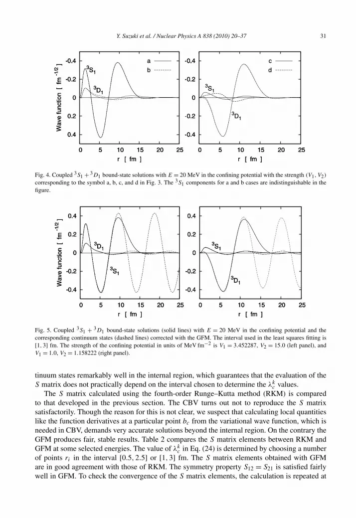
Fig. 5 compares the positive-energy bound states and the corresponding continuum states cor-rected by the GFM. The scattering energy is set to E = 20 MeV, and the two panels correspondto two different sets for the confining potential. The bound states wave functions follow the con-
Y. Suzuki et al. / Nuclear Physics A 838 (2010) 20–37 31
Fig. 4. Coupled 3S1 + 3D1 bound-state solutions with E = 20 MeV in the confining potential with the strength (V1,V2)
corresponding to the symbol a, b, c, and d in Fig. 3. The 3S1 components for a and b cases are indistinguishable in thefigure.
Fig. 5. Coupled 3S1 + 3D1 bound-state solutions (solid lines) with E = 20 MeV in the confining potential and thecorresponding continuum states (dashed lines) corrected with the GFM. The interval used in the least squares fitting is[1,3] fm. The strength of the confining potential in units of MeV fm−2 is V1 = 3.452287, V2 = 15.0 (left panel), andV1 = 1.0, V2 = 1.158222 (right panel).
tinuum states remarkably well in the internal region, which guarantees that the evaluation of theS matrix does not practically depend on the interval chosen to determine the λk
c values.The S matrix calculated using the fourth-order Runge–Kutta method (RKM) is compared
to that developed in the previous section. The CBV turns out not to reproduce the S matrixsatisfactorily. Though the reason for this is not clear, we suspect that calculating local quantitieslike the function derivatives at a particular point bc from the variational wave function, which isneeded in CBV, demands very accurate solutions beyond the internal region. On the contrary theGFM produces fair, stable results. Table 2 compares the S matrix elements between RKM andGFM at some selected energies. The value of λk
c in Eq. (24) is determined by choosing a numberof points ri in the interval [0.5,2.5] or [1,3] fm. The S matrix elements obtained with GFMare in good agreement with those of RKM. The symmetry property S12 = S21 is satisfied fairlywell in GFM. To check the convergence of the S matrix elements, the calculation is repeated at
32 Y. Suzuki et al. / Nuclear Physics A 838 (2010) 20–37
Table 2Comparison of the S matrix elements calculated with RKM and GFM for the proton–neutron scattering in the coupled3S1 +3 D1 states. The element written as a, b stands for a + ib. The square bracket denotes the interval in fm used inthe least squares fitting (27).
the same energies of the table by adopting a larger basis size with b0 = 0.05 fm, p = 1.25, andNB = 33. The difference between the two turns out to be very small.
It is also convenient to parametrize the S matrix in three real parameters δ1, δ2, εJ called thebar phase shifts and the mixing parameter,
S =(
exp(iδ1) 00 exp(iδ2)
)(cos 2εJ i sin 2εJ
i sin 2εJ cos 2εJ
)(exp(iδ1) 0
0 exp(iδ2)
). (42)
Fig. 6 compares the proton–neutron 3S1 + 3D1 bar phase shifts between the RKM and GFM.The agreement is good over the whole energy. We have repeated the calculation by changing theinterval to determine λk
c . The phase shifts are found to be stable.It is interesting to examine how well the GFM reproduces the S matrix at very low energy.
This is because obtaining the bound-state solutions with low energy may not be trivial in thebasis expansion method used here, as shown by the solvable-potential case. One has to eitherweaken the effect of the confining potential using a smaller strength Vc and/or a larger radiusdc or adopt more complete basis functions. The S matrix calculation becomes inaccurate belowE ≈ 1 MeV with the fourth-order RKM, so we instead use the Numerov method adapted to acoupled-channels case and compare to that obtained with the GFM. Fig. 7 displays the effective-range function, k1 cot δ1, for the 3S1 bar phase shift δ1, as a function of the wave number k1.The lowest energy reached with the GFM using dc = 9 fm is 20 keV, and the effective-rangefunction calculated with the GFM agrees very well with the Numerov results. We attempt to fitthe effective-range function with the “effective-range expansion” formula
k1 cot δ1 = −1 + 1r0k
21 − Pr3
0 k41 + · · · , (43)
a 2
Y. Suzuki et al. / Nuclear Physics A 838 (2010) 20–37 33
Fig. 6. Comparison of the bar phase shifts calculated with RKM and GFM for proton–neutron scattering in coupled3S1 + 3D1 states. The interval used in the least squares fitting is [1,3] fm.
Fig. 7. Comparison of the effective-range functions calculated with the Numerov method and the GFM for the 3S1 barphase shift of proton–neutron scattering as a function of the wave number.
to deduce the scattering length a and the effective range r0. Since the 3S1 and 3D1 channelscouple, it is noted that this expansion formula is in principle to be discussed on the basis ofthe eigenphase, defined in Eq. (41), but not of the bar phase [24]. We ignore this differencehere because our interest lies in testing the GFM at low energies. The values of a and r0 arededuced by the least squares fitting. When the fitting is made using the data in the energy range[0.02,1] MeV, we obtain a = 5.37 and r0 = 1.83 fm. Considering the fact that the G3RS potentialneither reproduces the deuteron ground-state energy nor the empirical phase shifts precisely,these values are in reasonable agreement with the experimental values, a = 5.424 ± 0.004, r0 =1.759 ± 0.005 [25] or a = 5.419 ± 0.007, r0 = 1.753 ± 0.008 fm as quoted in Ref. [26]. Todetermine the shape parameter P , we must use the expansion formula including higher orderterms in k1 than four, and may need to evaluate the effective-range function even more accurately.The above analysis demonstrates that the GFM enables us to determine the low energy S matrixaccurately.
The phase shifts for the proton–proton 3P2 + 3F2 scattering are displayed in Fig. 8. The GFMphase shifts are in satisfactory agreement with those of RKM, confirming that our method workswell in such a case that a long-range interaction like the Coulomb potential is present.
34 Y. Suzuki et al. / Nuclear Physics A 838 (2010) 20–37
Fig. 8. Comparison of the bar phase shifts calculated with RKM and GFM for proton–proton scattering in coupled3P2 + 3F2 states. The interval used in the least squares fitting is [0.5,2] fm.
4. Conclusion
Bound-state calculations can be performed accurately for a large variety of problems. Thedetermination of scattering states and in particular of the collision matrix does not always reachthe same level of precision. For this reason, a new method to obtain both the wave function andS matrix for coupled-channels scattering problems has been presented which allows using thewell established methods and codes developed for bound states. The method is characterized bythe introduction of real confining potentials only acting at distances where the potentials in thevarious channels are negligible. Several confining potentials, as many as the number of openchannels, are adjusted to provide different bound states at the considered scattering energy. Thelinear independence of the different solutions having the same energy is studied in terms of thestrength of the confining potentials. The asymptotic behavior of the continuum state is guaranteedin each channel with a single-channel Green’s function.
The feasibility and accuracy of the method are demonstrated by two examples. An exactlysolvable two-channel potential with unequal thresholds displaying a Feshbach resonance allowsus to show that the technique is as valid when some channels are closed as when they are allopen. In general, the eigenphase shifts and wave functions closely reproduce the exact solutions.The G3RS nucleon–nucleon potential provides a realistic example where we show the validityof the method over a wide range of incident energies including very low energies as well as inthe presence of the long-range Coulomb potential.
The discussion here presented is limited to the simple two-body case. The extension of themethod to describing scattering in a few-body system does not pose more difficulties than thoseinherent to the description of the corresponding bound states. In the particular case of the few-nucleon systems, several techniques are available for describing A � 4 bound states. Therefore,we expect that the present method will help in the description of few-nucleon scattering states.
Acknowledgements
The authors thank Y. Fujiwara for valuable communications and K. Nataami for his collab-oration at the late stage of this work. This study was performed as a part of the programme inthe agreement between the Japan Society for the Promotion of Science (JSPS) and the Fund forScientific Research of Belgium (F.R.S.-FNRS). Y.S. is supported by a Grant-in Aid for Scien-
Y. Suzuki et al. / Nuclear Physics A 838 (2010) 20–37 35
tific Research (No. 21540261). He is grateful to A. Bonaccorso for the invitation to Pisa in thesummer of 2009. This text presents research results of the Belgian program P6/23 on interuniver-sity attraction poles initiated by the Belgian-state Federal Services for Scientific, Technical andCultural Affairs (FSTC). D.B. also acknowledges travel support of the Fonds de la RechercheScientifique Collective (FRSC).
Appendix A. Regular and irregular solutions
We here summarize the regular and irregular solutions, v(r) and h(r), which are used in thepresent article. The differential equation which defines them is(
d2
dr2− �(� + 1)
r2− 2μ
h2U(r) + k2
)u(r) = 0, (A.1)
where k is assumed to be non-negative. The Green’s function G(r, r ′) is a solution to the equation(d2
dr2− �(� + 1)
r2− 2μ
h2U(r) + k2
)G
(r, r ′) = δ
(r − r ′), (A.2)
and it is given by
G(r, r ′) = v(r<)h(r>)/W(v,h), (A.3)
where r< (r>) is the lesser (greater) of r and r ′ and W(v,h) is the Wronskian. See Ref. [27] forthe definitions of special functions used here.
In the case where U(r) = 0, the solutions are expressed in terms of the spherical Besselfunctions of fractional order
The Wronskian is W(v,h) = −k. The outgoing wave is h(r) + iv(r) → (−i)�eikr for large r .In the case where U(r) = Z1Z2e
2/r , the solutions are expressed in terms of the Coulombwave functions
v(r) = F�(η, kr), h(r) = G�(η, kr), (A.5)
where the Sommerfeld parameter η is defined as μZ1Z2e2/h2k. The Wronskian is W(v,h) =
−k. The outgoing wave defined by h(r) + iv(r) approaches (−i)� ei(kr−η ln 2kr+σ�) for large r ,where σ� = argΓ (� + 1 + iη).
Appendix B. Bound-state solutions in confining potentials
The aim of this appendix is to discuss the relationship between the confining potentials andthe independent bound states which are constrained to have the same energy. Suppose that wehave another confining potential W = (Wc(r)) which has the same property as W , Eqs. (11)and (12). The function wc(r) is a solution to Eq. (13) with Wc(r) replaced by Wc(r), and givesenergy E (k2
c = 2μc(E − Ec)/h2). Temporarily we assume that E may not necessarily be equal
to E. To derive a necessary and sufficient condition that the two solutions (wc(r)) and (wc(r)) areindependent and have the same energy, we make use of the Wronskian, W(wc, wc). Its derivativereads
36 Y. Suzuki et al. / Nuclear Physics A 838 (2010) 20–37
h2
2μc
d
drW(wc, wc) = −{
Wc(r) − Wc(r)}wc(r)wc(r) + (E − E)wc(r)wc(r)
+∑c′
ac′∫0
Vcc′(r, r ′){wc(r)wc′
(r ′) − wc(r)wc′
(r ′)}dr ′, (B.1)
where use is made of Eq. (7) in the integration.Let bc be an arbitrary value in the interval [ac, dc]. Integrating Eq. (B.1) in [bc,∞] where
Vcc′ = 0, noting the function values at r = ∞ and summing over all the channels, we obtain arelation between Wronskians
∑c
h2
2μc
W(wc, wc)|r=bc =∑
c
∞∫dc
{Wc(r) − Wc(r)
}wc(r)wc(r) dr
− (E − E)∑
c
∞∫bc
wc(r)wc(r) dr. (B.2)
Here the lower limit of the integration in the first term on the right-hand side is set equal to dc
because both Wc(r) and Wc(r) vanish for r � dc. Performing a calculation similar to the above in[0, bc] and using the function values at r = 0, we obtain another expression for the same relationbetween Wronskians
∑c
h2
2μc
W(wc, wc)|r=bc =∑
c
∑c′
ac∫0
ac′∫0
Vcc′(r, r ′){wc(r)wc′
(r ′) − wc(r)wc′
(r ′)}dr dr ′
+ (E − E)∑
c
bc∫0
wc(r)wc(r) dr. (B.3)
With the help of the symmetry relation (6), the first term on the right-hand side of Eq. (B.3)vanishes. Thus the following identity is derived:
∑c
∞∫dc
{Wc(r) − Wc(r)
}wc(r)wc(r) dr = (E − E)
∑c
∞∫0
wc(r)wc(r) dr. (B.4)
Let us assume that the confining potential W gives the same energy as W , E = E. Then weimmediately obtain that W must satisfy a relation
∑c
∞∫dc
{Wc(r) − Wc(r)
}wc(r)wc(r) dr = 0. (B.5)
Conversely, if the two potentials W and W satisfy the condition (B.5), Eq. (B.4) shows that theyproduce the same energy or
∑c
∫ ∞0 wc(r)wc(r) dr = 0. The latter possibility is, however, very
unlikely except for an accidental case, thus leading to E = E.Suppose that W and W giving the same energy have different components, say in the chan-
nel c. Using Eq. (B.1) again leads to
Y. Suzuki et al. / Nuclear Physics A 838 (2010) 20–37 37
h2
2μc
W(wc, wc)|r=bc =∞∫
dc
{Wc(r) − Wc(r)
}wc(r)wc(r) dr. (B.6)
The right-hand side of the above equation is determined by dc alone. The Wronskian W(wc, wc)
is therefore independent of bc, that is, Eq. (B.6) is valid as long as bc ∈ [ac, dc]. Rewriting theWronskian as
W(wc, wc)|r=bc = wc(bc)wc(bc)
(w′
c(bc)
wc(bc)− w′
c(bc)
wc(bc)
), (B.7)
we assert that wc(r) and wc(r) must be different (independent) in the internal region providedW(wc, wc) does not vanish. This is because they have different logarithmic derivatives at bc,in spite of the fact that they are both solutions to the same equation (3) in the internal region,satisfying the vanishing condition at r = 0. Therefore Eq. (B.5) is a necessary and sufficientcondition that W and W give independent solutions to Eq. (13) with the same energy.
References
[1] A.U. Hazi, H.S. Taylor, Phys. Rev. A 1 (1970) 1109.[2] I.A. Ivanov, J. Mitroy, K. Varga, Phys. Rev. Lett. 87 (2001) 063201.[3] A.M. Lane, R.G. Thomas, Rev. Mod. Phys. 30 (1958) 257.[4] R.F. Barrett, B.A. Robson, W. Tobocman, Rev. Mod. Phys. 55 (1983) 155.[5] P. Descouvemont, D. Baye, Rep. Prog. Phys. 73 (2010) 036301.[6] M. Kamimura, Prog. Theor. Phys. Suppl. 62 (1977) 236.[7] P. Barletta, C. Romero-Redondo, A. Kievsky, M. Viviani, E. Garrido, Phys. Rev. Lett. 103 (2009) 090402;
A. Kievsky, M. Viviani, P. Barletta, C. Romero-Redondo, E. Garrido, Phys. Rev. C 81 (2010) 034002.[8] N. Moiseyev, Phys. Rep. 302 (1998) 211.[9] A.T. Kruppa, R. Suzuki, K. Kato, Phys. Rev. C 75 (2007) 044602.
[10] G. Jolicard, E. Austin, Chem. Phys. Lett. 121 (1985) 106.[11] U.V. Riss, H.-D. Meyer, J. Phys. B: At. Mol. Opt. Phys. 26 (1993) 4503.[12] R. Guérout, M. Jungen, C. Jungen, J. Phys. B 37 (2004) 3043;
R. Guérout, M. Jungen, C. Jungen, J. Phys. B 37 (2004) 3057.[13] J.Y. Zhang, J. Mitroy, K. Varga, Phys. Rev. A 78 (2008) 042705.[14] K.M. Nollett, S.C. Pieper, R.B. Wiringa, J. Carlson, G.M. Hale, Phys. Rev. Lett. 99 (2007) 022502.[15] S. Quaglioni, P. Navrátil, Phys. Rev. Lett. 101 (2008) 092501;
S. Quaglioni, P. Navrátil, Phys. Rev. C 79 (2009) 044606.[16] Y. Suzuki, W. Horiuchi, K. Arai, Nucl. Phys. A 823 (2009) 1.[17] H. Esbensen, C.N. Davids, Phys. Rev. C 63 (2000) 014315.[18] K. Varga, Y. Suzuki, Phys. Rev. C 52 (1995) 2885.[19] Y. Suzuki, K. Varga, Stochastic Variational Approach to Quantum-Mechanical Few-Body Problems, Lecture Notes
in Physics Monographs, vol. 54, Springer, Berlin, 1998.[20] E. Hiyama, Y. Kino, M. Kamimura, Prog. Part. Nucl. Phys. 51 (2003) 223.[21] J.R. Cox, J. Math. Phys. 5 (1964) 1065.[22] J.-M. Sparenberg, B.F. Samsonov, F. Foucart, D. Baye, J. Phys. A: Math. Gen. 39 (2006) L639.[23] R. Tamagaki, Prog. Theor. Phys. 39 (1968) 91.[24] J.M. Blatt, L.C. Biedenharn, Phys. Rev. 86 (1952) 399.[25] O. Dumbrajs, R. Koch, H. Pilkuhn, G.C. Oades, H. Behrens, J.J. de Swart, P. Kroll, Nucl. Phys. B 216 (1983) 277.[26] R. Machleidt, Phys. Rev. C 63 (2001) 024001.[27] M. Abramowitz, I.A. Stegun, Handbook of Mathematical Functions, Dover, New York, 1972.